Optimization of Neural Networks: A Comparative Analysis of the Genetic Algorithm and Simulated Annealing
Randall S. Sexton Department of Management Ball State University Muncie, Indiana 47306 Office (765) 285-5320 Fax (765) 285-8024 email
[email protected] Robert E. Dorsey, and John D. Johnson1 College of Business University of Mississippi University, Mississippi 38677 Office (601) 232-7575 Office (601) 232-5492 email
[email protected] email
[email protected]
1
Randall Sexton is an Assistant Professor in the College of Business, Ball State University. Robert Dorsey and John Johnson are Associate Professors in the College of Business, University of Mississippi. Dr’s Johnson and Dorsey are supported in part by the Mississippi Alabama Sea Grant Consortium through NOAA.
Optimization of Neural Networks: A Comparative Analysis of the Genetic Algorithm and Simulated Annealing
ABSTRACT
The escalation of Neural Network research in Business has been brought about by the ability of neural networks, as a tool, to closely approximate unknown functions to any degree of desired accuracy. Although, gradient based search techniques such as back-propagation are currently the most widely used optimization techniques for training neural networks, it has been shown that these gradient techniques are severely limited in their ability to find global solutions. Global search techniques have been identified as a potential solution to this problem. In this paper we examine two well known global search techniques, Simulated Annealing and the Genetic Algorithm, and compare their performance. A Monte Carlo study was conducted in order to test the appropriateness of these global search techniques for optimizing neural networks.
Keywords: Neural Networks; Optimization; Genetic Algorithm; Simulated Annealing; Global Solutions; Interpolation; Extrapolation
1
1. Introduction The explosion of business applications of artificial neural networks (ANN) is evidenced by the more than 400 citations referencing articles that have applied neural networks to business applications, within the last two years. This trend shows no signs of slowing as more researchers discover and begin to utilize this approximation tool. The ability of the ANN to accurately approximate unknown functions and their derivatives [8] [12], underlies this growing popularity. Because of its ease of use, an overwhelming majority of these applications have used some variation of the gradient technique, backpropagation [14][20][21] [30] for optimizing the networks [22]. Although, backpropagation has unquestionably been a major factor for the success of past neural network applications, it is plagued with inconsistent and unpredictable performances [1][13][15][16][21] [27][28][29][31]. Gradient search techniques such as backpropagation are designed for local search. They typically achieve the best solution in the region of their starting point. Obtaining a global solution is often dependent on a fortuitous choice of starting values. Global search techniques are known to more consistently obtain the optimal solution. Work in this area is summarized in [25] and specific applications can be found in [7], [19] and [26].
Recently, [24] demonstrated
that for a variety of complex functions the genetic algorithm was able to achieve superior solutions for neural network optimization than backpropagation and [23] found that another global search heuristic, Tabu Search (TS), is able to systematically achieve superior solutions for optimizing the neural network than those achieved by backpropagation. Although this literature demonstrates the superiority of global search to hill climbing techniques, the literature provides limited information about the relative performance of global search algorithms.
2
In addition to GA and TS another well known global search heuristic is simulated annealing. Simulated annealing has been shown to perform well for optimizing a wide variety of complex problems [10]. This paper compares the performance of these two well known global search algorithms, Simulated Annealing (SA) and the Genetic Algorithm (GA), for ANN optimization. The following section briefly describes the two global optimization techniques. The next section discusses the Monte Carlo experiment and results of the comparison. We then examine two real world problems to further show the benefits of global search techniques for neural network optimization and include a comparison with BP as well. The final section concludes.
2. The Search Algorithms The two global search techniques used for this study are briefly described in the following two sections. More detailed descriptions of these algorithms can be found in Dorsey and Mayer [5] for genetic algorithms and Goffe et al [10] for simulated annealing. 2.1 Genetic Algorithm The GA is a global search procedure that searches from one population of points to another. As the algorithm continuously samples the parameter space, the search is directed toward the area of the best solution so far. This algorithm has been shown to perform exceedingly well in obtaining global solutions for difficult non-linear functions [4] [5]. The application of the GA to one particularly complex non-linear function, the ANN, has also been shown to dominate other more commonly used search algorithms [6] [7].
3
A formal description of the algorithm is provided in [4], [5], [6] and [7]. Basically, an objective function, such as minimization of the sum of squared errors or sum of absolute errors, is chosen for optimizing the network. The objective functions need not be differentiable or even continuous. Using the chosen objective function, each candidate point out of the initial population of randomly chosen starting points is used to evaluate the objective function. These values are then used in assigning probabilities for each of the points in the population. For minimization, as in the case of sum of squared errors, the highest probability is assigned to the point with the lowest objective function value. Once all points have been assigned a probability, a new population of points is drawn from the original population with replacement. The points are chosen randomly with the probability of selection equal to its assigned probability value. Thus, those points generating the lowest sum of squared errors are the most likely to be represented in the new population. The points comprising this new population are then randomly paired for the crossover operation. Each point is a vector (string) of n parameters (weights). A position along the vectors is randomly selected for each pair of points and the preceding parameters are switched between the two points. This crossover operation results in each new point having parameters from both parent points. Finally, each weight has a small probability of being replaced with a value randomly chosen from the parameter space. This operation is referred to as mutation. Mutation enhances the GA by intermittently injecting a random point in order to better search the entire parameter space. This allows the GA to possibly escape from local optima if the new point generated is a better solution than has previously been found, thus providing a more robust solution. This
4
resulting set of points now becomes the new population, and the process repeats until convergence. Since this method simultaneously searches in many directions, the probability of finding a global optimum greatly increases. The algorithm’s similarity to natural selection inspires its name. As the GA progresses through generations, the parameters most favorable for optimizing the objective function will reproduce and thrive in future generations, while poorly performing parameters die out, as in “survival of the fittest”. Research using the GA for optimization has demonstrated its strong potential for obtaining globally optimal solutions [3] [11]. 2.2 Simulated Annealing Annealing, refers to the process which occurs when physical substances, such as metals, are raised to a high energy level (melted) and then gradually cooled until some solid state is reached. The goal of this process is to reach the lowest energy state. In this process physical substances usually move from higher energy states to lower ones if the cooling process is sufficiently slow, so minimization naturally occurs. Due to natural variability, however, there is some probability at each stage of the cooling process that a transition to a higher energy state will occur. As the energy state naturally declines, the probability of moving to a higher energy state decreases. A detailed description of the simulated annealing algorithm and its use for optimization can be found in [2]. In essence, simulated annealing draws an initial random point to start its search. From this point, the algorithm takes a step within a range predetermined by the user. This new point’s objective function value is then compared to the initial point’s value in order to determine if the new value is smaller. For the case of minimization, if the objective function
5
value decreases it is automatically accepted and it becomes the point from which the search will continue. The algorithm will then proceed with another step. Higher values for the objective function may also be accepted with a probability determined by the Metropolis criteria (see [2] or [10]). By occasionally accepting points with higher values of the objective function, the SA algorithm is able to escape local optima. As the algorithm progresses, the length of the steps declines, closing in on the final solution. The Metropolis criteria uses the initial user defined parameters, T (temperature) and RT (temperature reduction factor) to determine the probability of accepting a value of the objective function that is higher. Paralleling the real annealing process, as T decreases the probability of accepting higher values decreases. T is reduced by the function Ti+1 = RT*Ti, where I is the ith iteration of the function evaluation after every NT iterations. NT is the preset parameter which establishes the number of iterations between temperature reductions. For this study these three parameters were set to values suggested in the literature [2] [10]. Unlike the version of the GA used in this study in which all parameters are dynamically assigned by the algorithm, the performance of the SA algorithm depends on user defined parameters. Since the performance of the SA is significantly impacted by the choice of these parameters a range of values were used for three variables (T, RT, NT). We examine twelve different combinations in order to allow SA a full opportunity to obtain a global solution.
3. Monte Carlo Study The Monte Carlo comparison was conducted on the six test problems shown in equation 1. The functions for all problems are continuous and all are differentiable except number (3) which contains an absolute value. The GA was compared to twelve variations of the SA
6
algorithm. For the first five test problems, fifty observations were used as the training set. The data was generated by randomly drawing the inputs from the sets X1
[-100,100] and X2 [-
10,10]. In order to test the networks, two additional data sets, consisting of 150 observations each were also constructed. The first test set was generated to test the ability of the optimized ANN to interpolate. The interpolation test data was also drawn from the sets X1
[-100,100]
and X2 [-10,10], but did not include any common observations with the training set. The second test set was generated to evaluate the ability of the optimized ANN to extrapolate outside of the range of the training set. This data was drawn from X1
[-200,-101] and X1
[101,200]
and from X2 [-20,-11] and X2 [11,20]. The training data was normalized from -1 to 1 for both algorithms, in order to have identical training and output data for comparison. The same normalizing factor was used on the extrapolation data. The sum of squared errors (SSE) was used for optimization and the networks were compared on the basis of forecast error. Each network included 6 hidden nodes for all problems. A bias term was used on both the input and hidden layers so there were a total of 25 weights. There may well be better network architectures for the given problems, but since we are comparing the optimization methods, we chose a common architecture. The sixth problem consisted of a discrete version of the Mackey-Glass equation that has previously been used in neural network literature [9][10]. This chaotic series is interesting because of its similarity to time series found in financial markets. Because of its apparent randomness and many local optima, this function is a challenging test for global training algorithms. Again, we chose 6 hidden nodes for the neural network architecture. Five lagged values of the dependent variable were used as the input variables. Clearly, three of these were
7
unnecessary but this information is often not known to the researcher and the ability of the ANN to ignore irrelevant variables is critical to its usefulness. Since there are five input variables, the total number of parameters included 36 weights connecting the five inputs and one bias term to the hidden nodes and seven weights connecting the hidden nodes and bias term to the output node, totaling 43 parameters overall. The training set of 100 observations for problem six started from the initial point of [1.6, 0, 0, 0, 0]. The interpolation test data consisted of 150 points that were generated from the randomly chosen point [-0.218357539, 0.05555536, 1.075291525, -1.169494128, 0.263368033].
Experiment Problems
(1)
1) Y ' X1 % X2 2) Y ' X1X2 X1 3) Y ' *X2* %1 2
3
3
2
4) Y ' X1 & X2 5) Y ' X1 & X1
6) Yt ' Yt&1 % 10.5
.2Yt&5 1 % (Yt&5)10
& .1Yt&1
3.1 Training with Simulated Annealing The version of Simulated Annealing used in this study came from Goffe et al. [10]. This code, like the GA program was written in Fortran 77 and run on a Cray J-916 supercomputer. In training each problem using SA, there were three factors that were manipulated in an effort to find the best configuration for optimizing each problem. They included the temperature (T) at three levels, the temperature reduction factor (RT), and the number of function evaluations before temperature reduction (NT), each at two levels. The different combinations of these
8
factors were used in an attempt to try and find the best combination for SA to obtain the global solution. Other parameters that could have been adjusted were set to the recommended values in Goffe et al [10]. Specifically, the number of cycles (NS) was set to 20. After NS*N function evaluations, each element of VM (step size) is adjusted so that approximately half of all function evaluations are accepted. The number of final function evaluations (NEPS) was set to 4. This is used as part of the termination process. The error tolerance for termination was set to 10-6 and the upper limit for the total number of function evaluations (MAXEVL) was set to 10 9. Although this Monte Carlo study included the parameter settings recommended by both Goffe et al.[10] and Corana et al. [2], a more rigorous exploration of the parameters may have produced better performance for the SA. Table 1 below illustrates the specific parameter settings for each combination. Since the optimal solutions are not known a priori, the size of the search space was set between -600 and 600.
Table 1: Simulated Annealing Parameters Parameter
Values Used
Temperature (T)
5 50,000 50 Million
Temperature Reduction Factor (RT)
.50, .85
Number of Function Evaluations Before Temperature Reduction
5, Max(100, 5*N) N = The solution vector size.
Each of the twelve configurations was trained with ten replications. Each replication was started with new random seeds, thus there were 120 SA trials for each problem. The maximum number of function evaluations was set arbitrarily high (MAXEVL = 109) in order for all problems to terminate with the internal stopping rule based on the predefined error tolerance.
9
3.2 Training with the Genetic Algorithm The particular Genetic Algorithm used in this comparison was obtained from Dorsey et al. [7]. This program was also written in Fortran 77 and run on the CRAY J-916. This algorithm requires no preselection of parameters other than the number of hidden nodes, therefore only ten replications were run to test the effectiveness of this algorithm. Each replication differed only in the random initialization of the network. Each training replication was trained for 5,000 generations, which included a search of 20 points per generation. The same range for the parameter search [-600,600] was used as was used with SA. Although 5,000 generations did not allow full convergence for any of the six problems it was sufficient to demonstrate the effectiveness of this global search technique.
4. Results Since the structure of the ANN was held constant there were no additional parameters to adjust with the GA. Therefore, the test problems were only trained ten times each. The sole difference between each replication was the random initialization of the weights. The GA was terminated after 5000 generations as a base line for comparison with SA. A solution arbitrarily close to zero can be found given additional time for convergence. Although, the preset termination of the GA did not enable it to obtain the global solution, it provided a comparison point with the SA results for in-sample, interpolation and extrapolation data. In many cases, the GA’s worst in-sample solutions dominated the best SA results. The Mackey-Glass equation, problem 6, was the only problem in which the best GA solution was not superior to the best SA in-sample results. The best in-sample results for the GA and SA are shown in Table 2.
10
Table 2 - GA and SA Best and Worst In-Sample Comparisons Best and Worst Solutions for SA and GA Problems
GA
SA
Best
Worst
Best
Worst
1
4.16E-07
8.46E-06
1.05E-05
3.92E-03
2
1.27E-02
5.07E-01
3.17E-02
3.70E+00
3
1.82E-01
1.29E+00
1.77E+00
4.10E+00
4
4.09E-02
2.20E+00
4.84E-01
4.58E+01
5
2.90E-03
1.09E-00
4.39E-01
1.30E+01
6
2.53E-02
1.29E-01
1.02E-02
1.93E-01
Although, the twelve configurations of parameters for the SA included the recommended parameter settings of two previous studies [2] [10], none of the six test problems found an optimal solution with this configuration. In order to determine the best configuration, each test problem was initialized at ten different random points for all twelve configurations. Out of these one hundred twenty replications for each problem, the best solution so far was then chosen as the optimal configuration of the SA parameters for the particular test problem. However, since there were several other variables that could have been adjusted, as well as the infinite combination of possible levels for T, RT, and NT, we can not conclude that our configuration is the optimal configuration. A difficulty we experienced with SA is that there are no rules for adjusting the configuration to produce better results. Heuristics for setting SA parameters are suggested in [2] and [10] and the suggestion to set NT = 5 from [10] and NT = Max[100,5*N] from [2] can be followed, as was done in this study, but there is no guarantee that an optimal configuration for the algorithm will be found. In calculating Max[100, 5*N] for NT, only the number of input weights were used. SA only searched over these values, while the output weights were found
11
with OLS. The SA configurations that achieved the best and worst solutions out of the 120 different replications are shown in Table 3.
Table 3 - SA’s Best and Worst Configurations Best and Worst Configurations for SA Problems Best Worst T RT NT T 1 50,000 .5 100 50,000 2 50 M .85 100 50 M 3 50,000 .5 5 50,000 4 50,000 .5 100 50,000 5 50 M .5 5 50 M 6 5 .85 5 50,000
RT NT .5 5 .5 5 .5 5 .5 5 .5 5 .5 5
The best solutions, or sets of weights, for the in-sample data were then applied to out-ofsample interpolation and extrapolation data for each corresponding problem. Each data set consisted of 150 observations drawn uniformly from the ranges described earlier. Although SA had many more function evaluations, the GA obtained superior in-sample solutions in every case except problem six. A direct comparison of in-sample, interpolation and extrapolation results can be found in Table 4. The numbers shown in Table 4 are for the best solution of the ten runs for the GA and the best solution of the 120 runs for SA. The ANN solution dominated those of SA in every case for interpolation and extrapolation. Table 5 shows the processing time and number of function evaluations for the search techniques. Even though the GA was terminated prematurely, the solutions typically dominated the SA results despite the fact that the SA search involved far more function evaluations. The numbers shown in Table 5 are for the best solution of the ten runs for the GA and the best solution of the 120 runs for SA.
12
Table 4 - Best RMS Error Comparison for In-Sample, Interpolation, and Extrapolation Problems 1 2 3 4 5 6
IN-SAMPLE INTERPOLATION EXTRAPOLATION GA SA GA SA GA SA 4.16E-07 1.05E-05 3.68E-07 1.56E-05 6.74E-05 1.48E-04 1.27E-02 3.17E-02 1.72E-02 1.85E-01 0.869 7.42 1.82E-01 1.76 1.38 5.53 7.85 8.06 4.09E-02 4.84E-01 4.53E-02 2.73 7.40 234.26 3.06E-03 4.39E-01 2.02E-02 1.36 104.99 1647.81 2.53E-02 1.02E-02 3.40E-02 2.69E-01 NA NA
Table 5 - Time and Function Evaluation Comparison Problems Time on Number of Function Cray (sec) Evaluations 1 2 3 4 5 6
GA 53 53 122 122 113 181
SA 780 3,786 70 1,574 58 420
GA 100,000 100,000 100,000 100,000 100,000 100,000
SA 2,625,001 12,625,001 112,501 2,562,501 96,901 473,001
The SA estimates often diverge when estimating out-of-sample data. An examination of the solution weights revealed that in searching for a global solution, the SA algorithm typically reduced the complexity of the problems by often selecting negative and positive values that were very large in absolute terms. This caused the sigmoid function to output either 1 or 0 for many of the hidden nodes. For all six problems the SA algorithm chose weights for the in-sample data sets that caused at least three out of the six hidden nodes to output either 1’s, 0’s, or a combination of 1’s and 0’s. By converging on this type of local, the SA algorithm severally limited its out-of-sample estimation ability. When interpolation or extrapolation data was
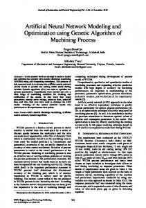
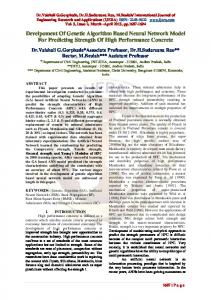
13
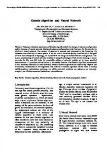
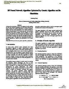
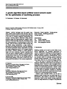
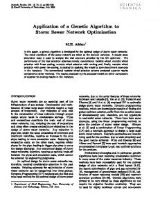
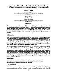
introduced that did not correspond with the given weights, it was unable to accurately forecast the data. Figures 1, 2, and 3 are XY graphs showing the true values forecasts from the ANNs trained with the two algorithms for problems 3, 4, and 6. The x-axis ranged from the 100th interpolation data point to the last data point in their respective interpolation data set. Both sets of forecasts tend to track the function for the interpolation data but the forecast from the SA trained ANN is very irregular. The GA trained ANN is relatively smooth thus allowing the derivative of the function to be more accurately computed and to better approximate the true function in general. Since the SA example obtained one run which found an in-sample solution superior to the one found by GA for problem 6 further exploration of the performance of the two algorithms on this problem seemed warranted. In addition to the architecture described above four other architectures were examined. These contained 2, 4, 8 and 10 hidden nodes. As before, for each case, ten replications were run, each starting from a different random seed. The genetic algorithm was trained for 15,000 generations and then terminated while the SA was allowed to run until it self terminated. The results are shown in Tables 6-9. As before, the average insample solution obtained by the GA was substantially better than that obtained by SA and the variation was also much smaller. The out of sample performance by the GA trained ANN dominated the performance of the SA trained ANN in every case. The one case reported earlier for the 6 hidden node SA trained ANN is still the best in-sample solution found but the best solutions found for the 8 and 10 hidden node cases by the GA are within 0.002 of that solution for the in-sample RMSE. The best out-of-sample results were again all obtained by the GA for all architectures.
14
Table 6: Average In-Sample Results for Problem 6 Hidden nodes GA RMSE SA RMSE GA StDev 2 1.33E-01 2.68E-01 2.48E-09 4 5.37E-02 1.34E-01 9.08E-07 6 3.38E-02 9.55E-02 6.46E-03 8 2.37E-02 7.93E-02 1.06E-02 10 2.29E-02 5.15E-02 1.10E-02
SA StDev 7.31E-02 4.53E-03 3.04E-02 1.16E-02 7.66E-03
Table 7: Average Out-of-Sample Results for Problem 6 Hidden nodes GA RMSE SA RMSE GA StDev 2 1.66E-01 3.41E-01 7.33E-08 4 6.89E-02 2.19E-01 2.24E-06 6 4.32E-02 4.04E-01 6.37E-03 8 3.19E-02 5.12E-01 1.16E-02 10 3.14E-02 6.45E-01 1.26E-02
SA StDev 9.23E-02 1.93E-02 1.18E-01 1.04E-01 8.74E-02
Table 8: Best Solutions for Problem 6 In-Sample Hidden nodes GA RMSE SA RMSE 2 1.33E-01 1.58E-01 4 5.37E-02 1.26E-01 6 1.75E-02 1.02E-02 8 1.19E-02 6.12E-02 10 1.16E-02 3.87E-02
Out-of-Sample GA StDev SA StDev 1.66E-01 2.00E-01 6.89E-02 2.05E-01 2.54E-02 2.69E-01 1.66E-02 4.41E-01 1.67E-02 6.42E-01
Table 9: Average CPU Time and Function Evaluations (FE) for Problem 6 Hidden nodes GA Time SA Time GA FE SA FE 2 193 132 300,000 171,841 4 437 622 300,000 463,201 6 681 **1,058 300,000 516,381 8 905 1,951 300,000 744,481 10 1,161 3,006 300,000 928,801 **This time was estimated PC seconds calculated from Cray CPU time.
15
5. Additional Comparison using a Classification and Time Series Problem Two additional real world problems were examined using GA, SA and BP. Since, the BP algorithm used in this comparison is PC based, the GA and SA programs were ported and optimized for a PC based 200MHz Pentium Pro using the NT 4.0 operating system. 5.1 Data Set Descriptions The first problem is a two group classification problem for predicting breast cancer [18]. This data set included 9 inputs that were constructed based on visual inspection by an experienced oncologist of possible cancerous cells. These values include, clump thickness, uniformity of cell size, uniformity of cell shape, marginal adhesion, single epithelial cell size, bare nuclei, bland chromatin, normal nucleioli, and mitoses. More detailed information on this data set can be found in [17] and [18]. The output value classified individuals as whether or not the patient’s breast lump was malignant and were set to the discrete values of -1 for nonmalignant and 1 for malignant. The original research classified this data using LP techniques for network optimization. This training data set included 369 records, each consisting of a nine dimensional input vector and corresponding output. The testing set included an additional 334 records. The data was downloaded from ftp.cs.wisc.edu in the directory /math-prog/cpodataset/machine-learn/. Since the training data set included more negative outputs than positive, the cutoff value for classification was adjusted based on the frequency in the training set, which moved the value from 0.0 to -0.112 on a [-1,1] scale. The network architecture was held constant at 6 hidden nodes for the GA, SA, and BP. Comparisons were made of total classification rate as well as type 1 and 2 errors. Type 1 error is defined as the event of assigning an observation to group 1 that should be in group 2, while the type II error involves assigning an observation to group 2 that
16
should be in group 1. In the current comparison we will refer to negative outcomes (nonmalignant) to group 1 and positive outcomes (malignant) to group 2. The second problem is a financial time series used to predict the following day’s S&P 500 index closing price. The 8 inputs included the previous daily percentage change of the close for the Dow Jones Industrial Average, close for the Dow Jones Transportation Average, total volume for the New York Stock Exchange, close for the Dow Jones 20 Bond Average, close for the Dow Jones utility Average, high for the S&P 500 index, low for the S&P 500 index, and the close for the S&P 500 index. The observations were drawn from January 4, 1993-December 13, 1996, using the first 800 observations for training and the last 200 observations for testing. The network architecture was held constant at 6 nodes in the hidden layer1. Comparisons were made based the 200 out-of-sample observations. The data for this problem was downloaded from the Journal of Computational Intelligence in Finance site at http://ourworld.compuserve.com/homepages/ftpub/dd.htm 5.2 Training with Backpropagation Commercial neural network software was evaluated in order to determine which package would provide the best estimates for the two problems. These included, Neural Works Professional II/Plus by NeuralWare, Brain Maker by California Scientific, EXPO by Leading markets Technologies and MATLAB by Math Works (using both the backpropagation and the Marquardt-Levenberg algorithms). Although the performance was similar for all programs, Neural Works Professional II/Plus, a PC-based neural network application seemed to give the
1
This architecture and selection of input variables are not proposed as being optimal for solving this problem but are used solely for comparisons of how well each algorithm achieved a minimal solution given the same data.
17
best estimates and was chosen for the test series. When training with BP, there are many parameters which can be manipulated. For this comparison the initial step size and momentum was set to 1 and 0.9, respectively. In order to better converge upon a solution during the training process the learning coefficient (Lcoef) parameter was set to the recommended value of 0.5. This parameter decreases the step size and momentum term by 0.5 for every 10,000 epochs in order to eliminate osculation. An epoch can be defined as one pass through the training set. The specific BP algorithm used was the Norm-Cum-Delta. The BP networks were trained for 1,000,000 epochs, at which time for every 10,000 additional epochs the error was checked to determine if a new solution was found that was smaller than the last. Termination of training occurred once there were 10 consecutive checks were there were no improvements. For each problem the BP networks were replicated 10 times starting each replication with a different random seed. 5.3 Training with Simulated Annealing The code for SA was ported and optimized for a PC-based machine so that results could be compared directly with the PC-based BP software. The recommended parameter values were used for both problems. Similar to BP, there were 10 replications, for each problem, using different random seeds for network initialization. The SA networks terminated once the training error tolerance reached 10-6 or maximum evaluations exceeded 109. 5.4 Training with the Genetic Algorithm The code for the GA was ported and optimized for a PC-Based machine to compare results directly with the BP and SA PC-based software. Ten replications were run, only changing the random seed for each replication. The number of generations for the GA was limited to 5,000, or in other words 100,000 function evaluations for each problem.
18
5.5 Classification Results Each of the algorithms was evaluated based on the total classification rate, as well as type 1 and type 2 classification errors. This rate is the average correct classifications for all 10 replications for each of the algorithms. In addition CPU time and the number of function evaluations for each algorithm are shown for each technique. Table 10 provides the data for all algorithms for both problems. As can be seen, the GA found superior classification rates. While, the GA found these solutions in a shorter time than SA, it took on average 22% longer to converge than BP. Although, BP converged on a solution faster, it converged upon inferior solutions. In comparing SA with BP for these two problems, SA’s total cumulative classification rate was the same as BP. BP found superior classification rates for Type 1 errors, while SA found superior classification rate for Type 2. These results do not indicate that BP is a superior algorithm for finding global solutions over SA. Since the only differences between the replications was the initial random draw of weights it is apparent that SA is greatly affected by the starting point of the search.
Table 10: Average Algorithm Comparisons for the Breast Cancer Problem Algorithm Total Classification Rate
GA
SA
BP
98.5%
97.2%
97.2%
Type 1 Error Rate
1.5%
3.1%
2.3%
Type 2 Error Rate
1.4%
1.6%
4.1%
100,000
493,635
1,174,000
618
4,812
497
Number of Function Evaluations CPU Time in seconds*
* CPU times were based on a 200MHz Pentium-Pro machine
19
5.6 Time Series Results The second comparison uses financial data to compare the three algorithms on their ability to estimate a time series problem. Specifically to estimate the S&P 500 index one day in the future. The mean RMSE, standard deviation of the RMSE, best solution RMSE, worst solution RMSE, number of function evaluations, and CPU time for the three algorithms are shown in Table 11. In every replication the GA found better solutions than BP. As shown in Table 11, the GA’s worst solution out of the ten replications was better than BP’s best solution. It can also be seen by looking at the standard deviations of the GA and BP, that both of these algorithms were consistent in obtaining consistent results across different replications. In the comparison between the GA and SA, the GA’s average RMSE was superior to SA’s average RMSE. In fact, the GA’s average RMSE was the same as the best SA’s RMSE. It is interesting to note for SA that the standard deviation was significantly higher than the other two algorithms. This may be due in part to a dependancy on the initial random draw of weights, and may be in part be due to the selection of parameter settings for the specific problem being estimated. Although, SA found 2 solutions that were better than the best BP solutions it failed to out perform BP on average. Table 11: Algorithm Comparisons for the Time Series Problem Mean RMSE (10 runs) Standard Deviation (10 runs) Best Solution
GA SA BP 7.11E-03 9.49E-02 7.83E-03 3.57E-03 6.58E-02 1.56E-05 7.06E-03 7.11E-03 7.80E-03
Worst Solution Number of Function Evaluations CPU time in seconds
7.16E-03 100,000 1,330
2.05E-01 580,348 9,396
7.85E-03 1,228,000 635
20
The Wilcoxon Matched Pairs Signed Ranks test was conducted to show the differences between each of the ten replications for each algorithm. Table 12 illustrates the number of replications for each comparison where an algorithm found significantly superior solutions, at the 0.01 level of significance, over another algorithm. As can be seen in this table the GA found superior solutions over BP in all ten replications. However, SA only found two solutions out of the ten replications that were significantly superior to BP. In comparing the GA with SA, the GA found 8 out of 10 solutions that were significantly better than SA, while the other two comparisons were not significantly different at the 0.10 level.
Table 12 - Statistical Comparisons Comparisons GA and SA GA and BP SA and BP
0.01 level GA SA 8 0 GA BP 10 0 SA BP 2 8
Above 0.01 2 0 0
6. Conclusions In order for researchers to utilize artificial neural networks as a highly versatile flexible form estimation tool, methods of global optimization must be found. The most frequently used algorithm for optimizing neural networks today is backpropagation. This gradient search technique is likely to obtain local solutions. Sexton et. al. [24], have recently demonstrated that the local solutions obtained by backpropagation often perform poorly on even simple problems when forecasting out of sample. Simulated annealing, a global search algorithm, performs better
21
than backpropagation, but is also uses a point to point search. Both BP and SA have multiple user determined parameters which may significantly impact the solution. Since there are no established rules for selecting these parameters, solution outcome is based on chance. The genetic algorithm appears to be able to systematically obtain superior solutions to simulated annealing for optimizing neural networks. These solutions provide the researcher with superior estimates of interpolation data. The genetic algorithm’s process of moving from one population of points to another enables it to discard potential local solutions and also to achieve the superior solutions in a computationally more efficient manner.
22
7. REFERENCES [1] Archer, N., & Wang, S., “Application of the Back Propagation Neural Network Algorithm with Monotonicity Constraints for Two-Group Classification Problems,” Decision Sciences, 1993, 24(1), 60-75. [2] Corana, A., Marchesi, M., Martini, C., & Ridella, S., “Minimizing Multimodal Functions of Continuous Variables with the ‘Simulated Annealing’ Algorithm,” ACM Transactions on Mathematical Software, 1987, 13, 262-80. [3] De Jong, K. A., “An Analysis of the Behavior of a Class of Genetic Adaptive Systems,” Unpublished Ph.D. dissertation, University of Michigan, Dept. of Computer Science, 1975. [4] Dorsey, R. E., & Mayer, W. J., “Optimization Using Genetic Algorithms,” Advances in Artificial Intelligence in Economics, Finance, and Management (J. D. Johnson and A. B. Whinston, eds.). Vol. 1. Greenwich, CT: JAI Press Inc., 69-91. [5] Dorsey, R. E., & Mayer W. J., “Genetic Algorithms for Estimation Problems with Multiple Optima, Non-Differentiability, and other Irregular Features,” Journal of Business and Economic Statistics, 1995, 13(1), 53-66. [6] Dorsey, R. E., Johnson, J. D., & Mayer, W. J., “The Genetic Adaptive Neural Network Training (GANNT) for Generic Feedforward Artificial Neural Systems,” School of Business Administration Working Paper, available at http://www.bus.olemiss.edu/johnson/compress/compute.htm. [7] Dorsey, R. E., Johnson, J. D., & Mayer, W. J., “A Genetic Algorithm for the Training of Feedforward Neural Networks,” Advances in Artificial Intelligence in Economics, Finance and Management (J. D. Johnson and A. B. Whinston, eds., 93-111). Vol. 1. Greenwich, CT: JAI Press Inc., 1994. [8] Funahashi, K., “On the Approximate Realization of Continuous Mappings by Neural Networks,“ Neural Networks, 2(3), 183-192, 1989. [9] Gallant, R. A. & White, H., “On Learning the Derivatives of an Unknown Mapping with Multilayer Feedforward Networks.” Artificial Neural Networks. Cambridge, MA: Blackwell Publishers, 1992, 206-23. [10] Goffe, W. L., Ferrier, G. D., & Rogers, J., “Global Optimization of Statistical Functions with Simulated Annealing,” Journal of Econometrics, 1994, 60, 65-99. [11] Goldberg, D. E., “Genetic Algorithms in Search, Optimization and Machine Learning,” Reading, MA: Addison-Wesley, 1989.
23
[12] Hornik, K., Stinchcombe, M., & White, H., “Multilayer Feed-Forward Networks are Universal Approximators,” Neural Networks, 2(5), 359-66, 1989. [13] Hsiung, J.T., Suewatanakul, W., & Himmelblau, D. M., “Should Backpropagation be Replaced by more Effective Optimization Algorithms? Proceedings of the International Joint Conference on Neural Networks (IJCNN), 1990, 7, 353-356. [14] LeCun, Y., “Learning Processes in an Asymmetric Threshold Network,” Disordered Systems and Biological Organization, 233-40. Berlin: Springer Verlag, 1986. [15] Lenard, M., Alam, P., & Madey, G, “The Applications of Neural Networks and a Qualitative Response Model to the Auditor’s Going Concern Uncertainty Decision,” Decision Sciences, 1995, 26(2), 209-27. [16] Madey, G. R., & Denton, J., “Credit Evaluation with Missing Data Fields,” Proceedings of the INNS, Boston, 1988, 456. [17] Mangasarian, O. L. (1993) “Mathematical Programming in Neural Networks,” ORSA Journal on Computing, 5(4), 349-360. [18] Mangasarian, O. L., Street, W. N., Wolberg, W. H. (1995). “Breast Cancer Diagnosis and Prognosis via Linear Programming,” Operations Research, 43(4), 570-577. [19] D. J. Montana and L. Davis, Training Feedforward Neural Networks using Genetic Algorithms, Proceedings of the Third International Conference on Genetic Algorithms, Morgan Kaufmann, San Mateo, CA, 1989, 379-384. [20] Parker, D. Learning Logic, “Technical Report TR-87,” Cambridge, MA: Center for Computational Research in Economics and Management Science, MIT, 1985. [21] Rumelhart, D., Hinton, G., & Williams, R., “Learning Internal Representations by Error Propagation,” In D. Rumelhart & J. McCleeland (Eds.), Parallel distributed processing: Explorations in the microstructure of cognition (Vol. 1). Cambridge, MA: MIT Press, 1986. [22] Salchenberger, L. M., Cinar, E. M., & Lash, N. A., “Neural Networks: A New Tool for Predicting Thrift Failures,” Decision Sciences, 23, 899-916. [23] Sexton, R., Allidae, B., Dorsey, R., and Johnson, J., “Global Optimization for Artificial Neural Networks: A Tabu Search Application,” forthcoming in European Journal of Operational Research [24] Sexton, R., Dorsey, R., & Johnson, J, “Toward a Global Optimum for Neural Networks: A Comparison of the Genetic Algorithm and Backpropagation,” forthcoming in Decision Support Systems
24
[25] J. D. Schaffer, D. Whitley and L. J. Eshelman, Combinations of Genetic Algorithms and Neural Networks: A Survey of the State of the Art, COGANN-92 Combinations of Genetic Algorithms and Neural Networks, IEEE Computer Society Press, Los Alamitos, CA, 1992, 1-37. [26] J. D. Schaffer, "Combinations of Genetic Algorithms with Neural Networks or Fuzzy Systems," Computational Intelligence: Imitating Life, J.M. Zurada, R.J. Marks, and C. J. Robinson, eds., IEEE Press, 1994, pp. 371-382. [27] Subramanian, V., & Hung, M.S., “A GRG@-based System for Training Neural Networks: Design and Computational Experience,” ORSA Journal on Computing, 1990, 5(4), 386-394. [28] Wang, S., “The Unpredictability of Standard Back Propagation neural Networks in Classification Applications,” Management Science, 1995, 41(3), 555-59. [29] Watrous, R. L., “Learning Algorithms for Connections and Networks: Applied Gradient Methods of Nonlinear Optimization,” Proceedings of the IEEE Conference on Neural Networks 2, San Diego, IEEE, 1987, 619-27. [30] Werbos, P., “The Roots of Backpropagation: From Ordered Derivatives to Neural Networks and Political Forecasting,” New York, NY: John Wiley & Sons, Inc., 1993. [31] White, H, “Some Asymptotic Results for Back-Propagation,“ Proceedings of the IEEE Conference on Neural Networks 3, San Diego, IEEE, 1987, 261-66.
25
Figure 1
Problem 3 - Interpolation 10
Forecast
5
Prob 3
0
GA
-5
SA
-10 -8
-6
-4
-2 0 True Values
2
4
6
Figure 2
Problem 4 - Interpolation 28000
Forecast
26000 24000
Prob 4
22000
GA
20000 18000 16000 16000 18000 20000 22000 24000 26000 True Values
SA
26
Figure 3
Problem 6 - Interpolation 0.4
Forecast
0.2 Prob 6 0 GA
-0.2
SA
-0.4 -0.6 -0.5 -0.4 -0.3 -0.2 -0.1 0 True Values
0.1
0.2