nodes to its left, namely the level-i descendents of v, that are not dead; ... if there is a free node (i.e., a node that does not have any ancestor or descendent that is.
A Constant-Competitive Algorithm for Online OVSF Code Assignment F.Y.L. Chin∗ H.F. Ting†
Y. Zhang‡
Department of Computer Science The University of Hong Kong Pokfulam Road, Hong Kong
Abstract Orthogonal Variable Spreading Factor (OVSF) code assignment is a fundamental problem in Wideband Code-Division Multiple-Access (W-CDMA) systems, which plays an important role in third generation mobile communications. In the OVSF problem, codes must be assigned to incoming call requests with different data rate requirements, in such a way that they are mutually orthogonal with respect to an OVSF code tree. An OVSF code tree is a complete binary tree in which each node represents a code associated with the combined bandwidths of its two children. To be mutually orthogonal, each leaf-to-root path must contain at most one assigned code. In this paper, we focus on the online version of the OVSF code assignment problem and give a 10-competitive algorithm, improving the previous O(h)-competitive result, where h is the height of the code tree, and also another recent constant-competitive result, where the competitive ratio is only constant under amortized analysis and the constant is never determined. Finally, we also improve the lower bound of the problem from 3/2 to 5/3.
1
Introduction
Wideband Code-Division Multiple-Access (W-CDMA) technology is one of the main technologies widely-developed in recent years for the implementation of third-generation (3G) cellular systems. We consider the well-studied problem of Orthogonal Variable Spreading Factor (OVSF) code assignment in W-CDMA systems [5, 7, 11, 12, 14]. OVSF is an implementation of CDMA wherein, before each signal is transmitted, the spectrum is spread according to a unique code, which is derived from an OVSF code tree. An OVSF code tree is a complete binary tree. Users have requests for different data rates, and the OVSF code tree accommodates these different requests by assigning codes at different levels of the code tree, with the root being at the highest level and representing the entire bandwidth of the wireless system. The code at any node other than the root denotes the bandwidth half that of its parent in the tree. In any legal assignment in the code tree, no two assigned codes lie on a single path from the root to a leaf, i.e., any two assigned codes are mutually orthogonal. The subset of nodes in the code tree, which forms a legal assignment, is called a code assignment. A node x is said to be free if there are no assigned nodes in every root-to-leaf path containing x, ∗
Supported by HK RGC grant HKU-7113/07E. Supported by HK RGC grant HKU-7045/02E. ‡ Current address: Institut f¨ ur Mathematik, Technische Universit¨ at, Berlin. †
1
and thus making x an assigned node would still result in a legal assignment. For convenience, we use the words “code” and “node” interchangeably. Fig. 1 is an example of an OVSF code tree with the code assignment represented by the darkened nodes marked as c, d, e, g and i. level 4
level 3
level 2
level 1 level 0
i
a
b
d c
g e
h
f
Figure 1: an example of OVSF code tree, solid circles are the assigned codes To illustrate the essence of the OVSF code assignment problem, consider the configuration shown in Fig. 1. Let Req(x) denote the request to which code x is assigned. Suppose a level-1 code request arrives followed by a level-2 code request. If code b were assigned to the first request, we would have to make two code reassignments before we can assign code a to the second request, e.g. assign code h to Req(b) (and thereby freeing b) and assign f to Req(c) (freeing c and consequently a). If, on the other hand, h were assigned to the first request, only one reassignment would be needed to satisfy the second request, i.e. assign f to Req(c), then assign code a to the second request. Since each reassignment requires processing overhead and may affect the quality of communications, a natural idea is to design algorithms to minimize the number of reassignments. Note that this problem will not be too difficult and can be solved optimally by a greedy strategy if codes were never released. However, when codes can be released, the code tree can be fragmented and many reassignments might be needed if a good assignment algorithm was not used. In general, an algorithm for OVSF code assignment is expected to handle a sequence σ = (C1 , C2 , . . . , Ck , . . .) of code operations over time, each operation Ck being either to request a code at a particular level or to release an assigned code. Note that, if the total bandwidth of any set of free codes is less than the bandwidth required by a code request, the new code request has to be withdrawn. The OVSF code assignment problem is hard, and the approach has often been to produce heuristics, whose performance is measured by the approximation (or competitive) ratio, which compares the cost of the algorithm to the cost of the optimal off-line scheme, where cost is the total number of assignments or reassignments done by the algorithm. The problem has been studied extensively recently. There are several variations of this problem, including: One-Step Off-line Code Assignment: Given a code assignment F and a new level-i code request r, find a code assignment F ′ , which satisfies the new request with a minimal number of reassignments. For this variation, Minn and Siu [11] gave a greedy algorithm, and Erlebach et al. [5] proved that this problem is NP-hard and gave an O(h)-approximation algorithm, where h is the height of the OVSF code tree. General Off-line Code Assignment: Given a sequence σ of code operations, find a sequence of code assignments such that the total number of reassignments is minimum, assuming the initial code tree is empty. This variation was proved to be NP-hard by Marco Tomamichel [13], who also gave an exponential-time algorithm for this variation. Online Code Assignment: The operations in the sequence σ = (C1 , C2 , . . . , Ck , . . .) arrive through time. At any time t > 0, we only know about the operations until t and have no information about any future operations Ct′ with t′ > t. Again, the problem is to find a sequence of code assignments such that the total number of reassignments is minimum. For this 2
variation, Erlebach et al. [5] gave an O(h)-competitive algorithm, where h is the height of the code tree. With resource augmentation, which means the online algorithm is allowed to use more bandwidth than the optimal scheme, a 4-competitive algorithm with a double-sized code tree was given in [5]. Using 1/8 extra bandwidth (less resource augmentation), Chin et al. [3] gave an 5-competitive algorithm. Recently, Foriˇsek et al. [6] gave an online algorithm whose competitive ratio is constant under amortized analysis. In their paper, there is no estimate about the size of the constant and the worst case can still be O(h). In this paper, we focus on the online OVSF code assignment problem. We first observe that the online algorithm in [5], which is O(h)-competitive, forces the assigned codes in the OVSF code tree into a single fixed format. As observed in [5], there are two worst-case single-formatrespecting configurations which make the performance of the algorithm in [5] poor, one which is bad (i.e. requires a reassignment at each level of the OVSF code tree) for code request but good (i.e. constant reassignments) for code release and the other which is bad for code release but good for code request. Interestingly, these two code configurations differ by only one code assignment (but differ much in their structure), and so there exists a sequence of alternating code requests and releases, each of which requires h code reassignments, and hence O(h) for the competitive ratio. By allowing two types of format with similar structure, we are able to give a 10-competitive algorithm, improving the previous O(h)-competitive result [5], and the amortized O(1)-competitive result [6]. The rest of this paper is organized as follows. Sections 2 and 3 give the preliminary and the basic idea of our algorithm. Section 4 introduces a 10-competitive algorithm. Section 5 gives the correctness proof of the algorithm. A new lower bound of the problem, improving the bound from 3/2 to 5/3, is presented in Section 6.
2
Preliminaries
Let T be an OVSF code tree with a legal assignment A. In our discussion, we assume that T is ordered. We say that node u is dead if either it is assigned or at least one of its descendent is assigned. We say that a level ℓ of T is compact if any node at level ℓ that is to the left of some dead node at ℓ is also dead. We say that A is compact if all levels of T are compact. The following lemma suggests that the assigned nodes in a compact assignment are sorted; if we scan the OVSF code tree from left to right, the levels of the assigned nodes are non-decreasing. Lemma 1. Suppose that the legal assignment A is compact. Let u be an assigned node at level i and v be an assigned node at level j where i < j. Then, the level-j ancestor au of u must be to the left of v. Proof. Since A is legal, au cannot be v. If au is to the right of v, the dead node u has some nodes to its left, namely the level-i descendents of v, that are not dead; a contradiction. Intuitively, we should make the assignments compact in order to fully utilize the bandwidth. There is a simple strategy to ensure compactness: To serve a level-ℓ code request r, we “append” it to the right-end of the list of dead nodes at ℓ, or more precisely, we assign to r the node u that is immediately after the last dead node, i.e., the rightmost dead node at ℓ. It is obvious that the resulting assignment is also compact. However, it may not be legal; although u does not have any assigned descendent (because it is not dead before the update), it may have some assigned ancestor. To solve the problem, we distinguish two kinds of levels. We say that a level ℓ is rich if there is a free node (i.e., a node that does not have any ancestor or descendent that is assigned) immediately after the last dead node at ℓ; otherwise, it is poor. Note that if ℓ is rich, 3
then the resulting assignment is still legal after assigning u to r. Suppose that ℓ is poor. Then, u is not free and it must have an ancestor v assigned to some request Req(v). After assigning u to r, we need to reassign Req(v), i.e., freeing v followed by a code request Req(v), to make sure the assignment is legal. Note that this may trigger other reassignments of requests at higher levels. The following simple algorithm describes formally how this simple approach serves a level-ℓ request r. It makes use of two procedures AppendRich and AppendPoor. Let u be the node immediately after the last dead node at level ℓ. Procedure AppendRich(ℓ, r) is used when ℓ is rich; it simply assigns u to request r. Procedure AppendPoor(ℓ, r) is for the case when ℓ is poor. After assigning u to r, AppendPoor(ℓ, r) frees the assigned ancestor a of u, and returns the request to which a is assigned before it is freed. It is easy to see that both AppendRich and AppendPoor make one assignment and thus their cost is 1. 1: while ℓ is poor do 2: rg = AppendPoor(ℓ, r); {rg is a level-g request.} 3: ℓ = g; r = rg ; 4: end while 5: AppendRich(ℓ, r);
3
Some ideas for improvement
Note that the simple algorithm given in Section 2 might make a large number of calls to AppendPoor, and hence make a lot of (re)assignments, to serve a request. The following lemma is the key for reducing the number of (re)assignments. Lemma 2. Suppose ℓ is poor. After executing AppendPoor(ℓ, r), ℓ becomes rich. Proof. Note that if the last dead node u at ℓ is the left son of its parent p, then ℓ must be rich. It is because the right son v of p, which is immediately after u, must be free; v is not dead (because u is the last dead node) and hence has no assigned descendent, and u and v share the same set of ancestors and thus v does not have any assigned ancestor. Thus, if ℓ is poor, node u must be a right son. After AppendPoor(ℓ, r), the node after u, which is a left son, becomes the new last dead node of ℓ. As argued above, ℓ becomes rich. Note that if we call AppendPoor m times, then m levels will be changed from poor to rich. This is good because the next time we serve any request on these rich levels, we just need a simple assignment. The problem is that there might be no more requests on these levels, and the effort is wasted. To overcome the difficulty, we propose a lazy approach. Here is the idea. Suppose that there is a level-ℓ request r, and the levels ℓ, ℓ + 1, . . . , k − 1 are all poor, and level k is rich. Then, we will call AppendPoor k − ℓ times and then call AppendRich once. Our lazy approach will not make these k − ℓ calls for AppendPoor; instead, it jumps to the last step, calling AppendRich to assign the node u after the last dead node at k to the level-ℓ request r.1 Later, if there is some request on some level g ∈ [ℓ, k], we will do the necessary work that we have avoided previously in order to recover the correct free node at g and assign it to the request. To summarize, the lazy approach also aims at maintaining compact assignments. However, there may be some nodes that are assigned to some lower-level requests; we call these nodes partially assigned nodes. These partially assigned nodes induce some structures called tanks of 1
We are generous here by assigning a level-k node to a level-ℓ request. If we insist that a level-ℓ node must be assigned to r, then we can actually assign a level-ℓ descendent of u to r.
4
free nodes, or simply tanks, which are intervals [ℓ, k] of levels with the following properties: The level ℓ, ℓ + 1, . . . , k − 1 are all poor and the assigned nodes at these levels are all fully assigned. For level k, the last dead node of k is partially assigned to a level-ℓ request, and the remaining assigned nodes are fully assigned. We say that ℓ is the bottom of the tank [ℓ, k], and k is its top. It is not difficult to implement the lazy approach in such a way that the number of (re)assignments needed for serving a request can be reduced substantially. However, to achieve a constant number of (re)assignments, we need to impose two extra structural properties on tanks. The first property is about the top of tanks. Given any level ℓ, we say that ℓ is locally rich if the last dead node at ℓ is a left son of its parent. The following fact is easy to verify from the definition and the proof of Lemma 2. Fact 1. A locally rich level is a rich level. Suppose ℓ is locally rich. Then after executing AppendRich(ℓ, r), ℓ is no longer locally rich. If ℓ is poor, then after executing AppendPoor(ℓ, r), ℓ becomes locally rich. The first property on tanks that we need to maintain is the following: The top of every tank must be locally rich. To describe the second structural property, we consider two tanks [bo , to ] and [b1 , t1 ]. Suppose that [bo , to ] is below [b1 , t1 ], i.e, to < b1 . We say that the two tanks are merge-able if (i) all the levels between them, i.e., levels to + 1, to + 2, . . . , b1 − 1, are empty, i.e., the levels do not have any assigned nodes, and (ii) the last dead node at level to is the leftmost level-to descendent of its level-b1 ancestor. We find that merge-able tanks are bad for our approach. Therefore, our updating procedure will merge any two merge-able tanks as soon as they appear. In other words, our algorithm keeps the following invariant: (∗)
There is no merge-able tank in the assignment.
As can be seen in Figure 2, it is easy to merge two merge-able tanks using two (re)assignments, and the merging preserves the compactness of the assignment.
tank [b1,t1]
tank [bo,to]
Figure 2: Merging of two tanks
4
A lazy algorithm
In this section, we describe the algorithm LAZY, which implements the lazy approach efficiently. To simplify the description, we regard a locally rich level ℓ that does not belong to any tank is a tank [ℓ, ℓ] itself. Furthermore, when there is no confusion, we will add a subscript to a request to indicate its level, e.g., the request rg is a level-g request. In addition to AppendPoor and AppendRich, LAZY also makes use of the following two procedures. • FreeTail(ℓ): The level ℓ must not be empty. The procedure frees the last assigned node u at ℓ and returns the request to which u is assigned. • ReAssign(r, r ′ ): Here, r is a request in the assignment, and r ′ is one that is not in the assignment. Suppose that u is assigned to r. Then, the procedure frees u from r, and then assigns u to r ′ . 5
We are now ready to describe LAZY. We first describe how it serves a code request. Then, we explain how it releases a code.
4.1
Serving a level-ℓ request rℓ
We have three different cases to consider. Case 1: ℓ is poor and does not belong to any tank. Let h be the lowest level above ℓ that either belongs to some tank, or is rich. If there is no such h, we report not enough bandwidth (and we will prove in Section 5 that this is true). Note that if h does not belong to any tank, then h is rich, but not locally rich (otherwise, [h, h] itself is a tank). In such case, we simply call AppendRich(h, rℓ ). It can be verified that afterwards, h is locally rich and [ℓ, h] becomes a tank. To ensure (∗), we merge, if there is any, the merge-able tanks above or below [ℓ, h]. Thus, the total number of (re)assignments is at most 5. The case when h belongs to some tank is more complicated. In such case, h must be the bottom of this tank [h, t]. By definition, the last assigned node at level t is partially assigned to a level-h request rh . To serve rℓ , we first recover the free node at h by re-assigning rh back to h. Then, we insert rℓ to a level lower than h so that the (re)assignments can make use of the free node at h and stop. 1: if h 6= t then 2: rh = FreeTail(t); {t becomes rich} 3: rg = AppendPoor(h, rh ); AppendRich(t, rg ); {[g, t] becomes tank} 4: end if 5: {At this point, h is not empty and is locally rich (Fact 1)} 6: Let k be the highest level below h that is not empty. 7: If (k < ℓ) then let k = ℓ. 8: s = AppendPoor(k, rℓ ); {s must be from h and [ℓ, k] becomes tank.} 9: AppendRich(h, s); 10: {From Fact 1, h is not locally rich and thus [h, h] is not a tank.} It can be verified that the update needs at most 4 (re)assignments. Note that the additional tanks [g, t] and [ℓ, k] may be created. To ensure (∗), we need to do some tank mergings. As pointed out in Line 10, [h, h] is not a tank. Furthermore, there is no merge-able tank above [g, t] (because (∗) ensures there is none above [h, t] before the update). Therefore, we only need to merge tank below [ℓ, k], which requires two extra (re)assignments. Thus, we need at most 6 assignments to serve request r. However, note that if we need to merge [ℓ, k] with a tank below it, we can save the assignment used by AppendPoor(k, rℓ ) at Line 8; rℓ will be reassigned during the merging. This reduces the number of (re)assignments to 5. Case 2: ℓ is poor and belongs to some tank [b, t]. For this case, we insert rℓ to ℓ directly, and the tank [b, t] may be broken into two tanks, one above, and one below ℓ. 1: rg = AppendPoor(ℓ, rℓ ); {ℓ becomes locally rich.} 2: rb = FreeTail(t); AppendRich(t, rg ); {[g, t] becomes tank.} 3: {We have served rℓ successfully, but there is no node assigned to rb } 4: if b = ℓ then 5: AppendRich(ℓ, rb ); {Now, ℓ is not locally rich} 6: else 7: Let k be the highest level below ℓ that is not empty. 8: If (k < b) then let k = b. 9: s = AppendPoor(k, rb ); {s must be from ℓ and [b, k] becomes tank.} 10: AppendRich(ℓ, s); {Now, ℓ is not locally rich.} 11: end if
6
It can be verified that the total number of (re)assignments made is at most 4. Since ℓ is not locally rich, [ℓ, ℓ] is not a tank, and as guaranteed by (∗), there is no merge-able tanks above t or below b before the update. Therefore, [g, t] and [ℓ, k] have no merge-able tank above or below them, and this case does not need any tank merging. Case 3: ℓ is rich. For this case, we do the followings. if ℓ does not belong to any tank then AppendRich(ℓ, rℓ ); 3: else 4: {for this case ℓ belongs to a tank, and since ℓ is rich, it is the top of some tank [b, ℓ].} 5: if b = ℓ then 6: AppendRich(ℓ, rℓ ) 7: else 8: rb = FreeTail(ℓ); AppendRich(ℓ, rℓ ); 9: Let k be the highest level below ℓ that is not empty. 10: If (k < b) then let k = b. 11: s = AppendPoor(k, rb ); AppendRich(ℓ, s); 12: end if 13: end if It can be verified that after the possible merging of tanks, the total number of (re)assignments made is at most 5. Note that our algorithm uses AppendPoor and AppendRich to append a request after the last dead node of a level, and whenever we free a node, we will immediately assign it to some other request. Therefore, the compactness of the resulting assignment is preserved. 1:
2:
4.2
Release of a level-ℓ node assigned to request r
We first consider the case when ℓ is not in any tank. Then, ℓ is not locally rich; otherwise, [ℓ, ℓ] itself is a tank. For this case, we do the following: 1: rℓ = FreeTail(ℓ); 2: if r 6= rℓ then ReAssign(r, rℓ ); From the fact that ℓ is not locally rich before the update, it can be verified that the resulting assignment is still compact. Together with the two possible tank mergings, the update makes at most 5 (re)assignments. We now consider the case when ℓ is in some tank [b, t]. To release r, we do the following: 1: rb = FreeTail(t); 2: if b = ℓ then 3: if r 6= rb then ReAssign(r, rb ); 4: else 5: Let k be the highest level below ℓ that is not empty. 6: If (k < b) then let k = b. 7: s = AppendPoor(k, rb ); {s must be from ℓ, and [b, k] becomes tank.} 8: if r 6= s then ReAssign(r, s); 9: end if Note that after the execution, the assignment may not be compact; we have freed the last assigned node at level t and did not reassign the node to any request. This may create some hole, i.e., free node, between two dead nodes at some levels above t. In such case, we need to fill up the hole as follows. Let z be the lowest level above t that is not empty, and vhole be the 7
free node, if any, created at level z. Note that by (∗), there is no merge-able tank above [b, t]; this implies z is not in any tank, and it is not locally rich. The following two steps will restore the compactness of the assignment: 1: rz = FreeTail(z); {z is now locally rich} 2: Assign vhole to rz . It is important to note that freeing the last assigned node u at level z will not create any problem; since z is not locally rich, u must be the right son of its parent p. After freeing u, p is still dead because its left son is dead. It can be verified that the whole release procedure, together with possible tank mergings, uses at most 5 (re)assignments in the worst case. The following theorem summarizes our discussion in this section. Theorem 1. Let A be a compact assignment satisfying (∗). LAZY serves any code request or code release for A using at most 5 (re)assignments. The resulting assignment is still compact and satisfies (∗). Furthermore, LAZY is 10-competitive. Proof. To see that LAZY is 10-competitive, suppose that there are m1 code requests and m2 code releases. Obviously, m2 ≤ m1 . To serve these requests and releases, LAZY makes at most 5m1 + 5m2 ≤ 10m1 (re)assignment. Note that the optimal algorithm has to make at least m1 assignments for the m1 code requests. The theorem follows.
5
LAZY fully utilizes the bandwidth
In this section, we prove that LAZY fully utilizes the bandwidth. More precisely, we prove that if LAZY cannot find an assignment to satisfy all the requests, then no assignment can satisfy these requests. First, we need to define the notion of leaf capturing. A node that is fully assigned captures all of its leaf descendents. A node that is partially assigned to a level-ℓ request captures its leftmost 2ℓ leaf descendents. For any node u, define F (u) to be P the set of leaf descendents of u that are not captured. For any set X of nodes, define F (X) = u∈X F (u). Intuitively, for the root r, F (r) is the remaining bandwidth not used by the current assignment. It is important to note that for a fixed set L of code requests, different legal assignments for L have the same value of F (r). Lemma 3. Let A be an assignment maintained by LAZY, and for any level ℓ, let Dℓ be the set of dead nodes at level ℓ. Then, |F (Dℓ )| < 2ℓ . Proof. The lemma is obviously true for level 0. Suppose it is true for all levels below ℓ, and we consider the level ℓ. Let u1 , u2 , . . . , uk be the sequence of dead nodes at ℓ where uk is the last dead node. First, we assume that there is no partially assigned node at ℓ. Let ui be the last node that is not assigned. Then, F (Dℓ ) = F ({u1 , u2 , . . . ui }) + F ({ui+1 , . . . , uk }). Since ui is the last node not assigned, ui+1 , . . . , uk are all assigned and the second term F ({ui+1 , . . . , uk }) is zero. To estimate the first term, let w be the last dead node at level ℓ − 1. Note that w must be a child of ui ; it cannot be a child of the nodes to the left of ui because these nodes are either assigned or not dead, and it cannot be a child of u1 , . . . , ui−1 , otherwise ui is not dead (recall that ui is not assigned). If w is the right child of ui , then F ({u1 , . . . , ui }) = F (Dℓ−1 ); otherwise F ({u1 , . . . , ui }) = F (Dℓ−1 )+2ℓ−1 . Together with the induction hypothesis that F (Dℓ−1 ) < 2ℓ−1 , the lemma follows. We now suppose that there is a partially assigned node at ℓ. According to LAZY, we conclude that the last dead node uk is the only partially assigned node at ℓ. Suppose that it is partially assigned by a level-g request. Then, [g, ℓ] is a tank and the levels g, g + 1, . . . , ℓ − 1 are all poor. 8
Let w1 , w2 , . . . , wm be the sequence of level-g descendents of u1 , u2 , . . . , uk−1 . Then, F (Dℓ ) = F (u1 , . . . , uk−1 ) + F (uk ) = F (w1 , . . . , wm ) + F (uk ) = F (w1 , . . . , wi ) + F (wi+1 , . . . , wm ) + F (uk ) where wi is the last dead node at level g. By the induction hypothesis, we conclude that F (Dg ) = F ({w1 , . . . , wi }) < 2g , and by the definition of captured leaves for partially assigned node, we have F (uk ) = 2ℓ − 2g . In the rest of the proof, we show that F (wi+1 , . . . , wm ) = 0 and the lemma follows. Suppose to the contrary that F (wi+1 , . . . , wm ) > 0. Then, among the leaf descendents of wi+1 , . . . , wm , there is one that is not captured. Let w and u be respectively the level-g and level-ℓ ancestors of this leaf. Note that w is to the right of wi and hence is not dead, and u is to the left of uk and hence is dead . Let d be the last dead node along the path from u down to w. Suppose that d is at level h. It follows that its left child vleft must be dead, and its right child vright , which must be along the path from u to w, is not dead (because d is the last dead node on this path). Since vleft is dead, none of its ancestors is assigned, and since vright is not dead, none of its descendent is assigned. Note that vleft and vright has the same set of ancestors and it follows that vright is free. Therefore, we conclude that at level h − 1, where g ≤ h − 1 ≤ ℓ − 1, there is a free node vright following the dead node vleft , and thus h − 1 is not poor; a contradiction. Theorem 2. Suppose that LAZY reports “not enough bandwidth” when serving a level-ℓ request r. Let L be the set of requests in the current assignment. Then, there is no assignment that can safisfy all the requests in L ∪ {r}. Proof. LAZY reports “not enough bandwidth” because level ℓ, as well as all levels above ℓ are poor. Let u1 , u2 , . . . , ui be the sequence of dead nodes, and ui+1 , . . . , um be the remaining nodes, at ℓ. Then there are F ({u1 , . . . , ui }) + F ({ui+1 , . . . , um }) leaves that are not captured. By Lemma 3, we conclude that F ({u1 , . . . , ui }) < 2ℓ . Since all levels above ℓ are poor, we can use an argument similar to the one used in the proof of Lemma 3 that F ({ui+1 , . . . , um }) = 0. It follows that F ({u1 , u2 . . . , um } < 2ℓ . Since assigning any node to r needs to capture 2ℓ leaves, there is no assignment can satisfy all requests L ∪ {r}.
6
Lower Bound
In [5], it is shown that the competitive ratio of any online algorithm for the code assignment problem must be at least 1.5. The following theorem shows that this bound can be improved to 5/3 by modifying the main idea given in [5]. Theorem 3. No deterministic algorithm can solve the online code assignment problem better than 5/3-competitive. Proof. Consider a code tree with N leaves (leaf-codes) and a sequence of level-0 code requests with each request assigned to each leaf code one by one. As soon as both right and left subtrees of the root have at least N/4 assigned leaf codes, the adversary will stop issuing any more level-0 code requests. Thus there will be at most 3N/4 level-0 code requests in the sequence. Then the adversary will repeatedly release those requests in the subtree with more than N/4 assigned leaf codes until both subtrees have exactly N/4 assigned leaf codes. The adversary will then make a level-(n − 1) request which will cause at least N/4 code reassignments, which end up with either the right or the left subtree with full assigned leaf codes. The adversary will then proceed recursively with the subtree with full assigned leaf codes by releasing its every other node. This process will be repeated log2 N − 1 times with a total of N/2 − 1 reassignments. On the other 9
hand, the optimal algorithm can assign the leave codes in such a way that no extra reassignments will be needed. Thus the optimal algorithm will take no more than 3N/4+log 2 N −1 assignments, whereas the adversary will take a total of 5N/4 + log 2 N − 2 (re)assignments. As a consequence, the competitive ratio will tend to be 5/3 asymptotically. Acknowledgements. The authors thank Dr. Bethany M. Y. Chan for her efforts in making this paper more readable.
References [1] W.T. Chan, F.Y.L. Chin, D. Ye, Y. Zhang and H. Zhu. Frequency Allocation Problem for Linear Cellular Networks. In Proc. of the 17th Annual International Symposium on Algorithms and Computation (ISAAC 2006), LNCS 4288, 61–70. [2] W.T. Chan, F.Y.L. Chin, D. Ye, Y. Zhang and H. Zhu. Greedy Online Frequency Allocation in Cellular Networks. Information Processing Letters, 102(2-3):55–61, April, 2007. [3] F.Y.L. Chin, Y. Zhang and H. Zhu. Online OVSF Code Assignment in Cellular Networks. In proc. of the 3rd International Conference on Algorithmic Aspects in Information and Management (AAIM 07), pp. 191–200, June, 2007. [4] I. Caragiannis, C. Kaklamanis, and E. Papaioannou. Efficient on-line frequency allocation and call control in cellular networks. Theory Comput. Syst., 35(5):521–543, 2002. A preliminary version of the paper appeared in SPAA 2000. [5] T. Erlebach, R. Jacob, M. Mihalak, M. Nunkesser, G. Szabo and P. Widmayer. An algorithmic view on OVSF code assignment. In proc. of the 21st Symposium on Theoretical Aspects of Computer Science (STACS 2004), LNCS 2996, pp. 270–281. [6] M. Foriˇsek, B. Katreniak, J. Katreniakov´a, R. Kr´ aloviˇc, R. Kr´ alovicˇc, V. Koutn´ y, D. Pardubsk´a, T. Plachetka and B. Rovan. Online bandwidth allocation. In proc. of the 16th Annual European Symposium on Algorithms (ESA2007), to appear. [7] X.Y. Li and P.J. Wan. Theoretically Good Distributed CDMA/OVSF Code Assignment for Wireless Ad Hoc Networks. In Proc. the 11th Annual International Conference of Computing and Combinatorics (COCOON05), pp. 126–135. [8] D.E. Knuth. The Art of Computer Programming, Volume 1: Fundamental Algorithms, AddisonWesley, 1975. [9] B. Kalyanasundaram and K. Pruhs. Speed is as powerful as clairvoyance. In Proceedings of the 36th IEEE Symposium on Foundations of Computer Science, pages 214–221, 1995. [10] C. McDiarmid and B.A. Reed. Channel assignment and weighted coloring. Networks, 36(2):114–117, 2000. [11] T. Minn and K.Y. Siu. Dynamic assignment of orthogonal variable-spreading factor codes in WCDMA. IEEE Journal on Selected Areas in Communications, 18(8):1429–1440, 2000. [12] A.N. Rouskas and D.N. Skoutas. OVSF codes assignment and reassignment at the forward link OFW-CDMA 3G systems. In Proc. of the 13 th IEEE International Symposium on Personal, Indoor and Mobile Radio Communications. [13] T. Erlebach, R. Jacob and Marco Tomamichel. Algorithmische Aspekte von OVSF Code Assignment mit Schwerpunkt auf Offline Code Assignment. Student thesis at ETH Z¨ urich. [14] P.J. Wan, X.Y. Li and O. Frieder. OVSF-CDMA Code Assignment in Wireless Ad Hoc Networks. In Proc. of DIAL M-POMC 2004 joint workshop on Foundations of mobile computing, pp. 92-101, 2004.
10