Srinivas Peeta and Debjit Das
1
A Continuous Learning Framework for Freeway Incident Detection Srinivas Peeta Debjit Das School of Civil Engineering Purdue University West Lafayette, IN 47907 (765) 494-2209 (765) 496-1105 (FAX)
[email protected] [email protected] ABSTRACT Existing freeway incident detection algorithms predominantly require extensive off-line training and calibration precluding transferability to new sites. Also, they are insensitive to demand and supply changes in the current site without recalibration. We propose two neural network based approaches that incorporate an on-line learning capability, thereby ensuring transferability, and adaptability to changes at the current site. The Least Squares technique and the Error Back Propagation algorithm are used to develop on-line neural network trained versions of the popular California algorithm and the more recent McMaster algorithm. Simulated data from the INTRAS model is used to analyze the performance of the neural network based versions of the California and McMaster algorithms over a broad spectrum of operational scenarios. The results illustrate the superior performance of the neural net implementations in terms of detection rate (DR), false alarm rate (FAR), and time to detection (TTD). Of implications to current practice, they suggest that just introducing a continuous learning capability to commonly employed detection algorithms in practice such as the California algorithm enhances their performance with time in service, allows transferability, and ensures adaptability to changes at the current site. An added advantage of this strategy is that existing traffic measures used (such as volume, occupancy, etc.) in those algorithms are sufficient, circumventing the need for new traffic measures, new threshold parameters, and/or variables requiring subjective decisions. KEYWORDS Incident detection, Neural Networks, Continuous learning. TRB Paper Number: 980962 Word Count: 4738 Number of Figures: 11
INTRODUCTION
Srinivas Peeta and Debjit Das
2
Automatic incident detection is an important component of a freeway traffic management system. Though several approaches have been proposed to date, no consensus exists on a particular algorithm as being the most appropriate. Traditional approaches have not been able to achieve consistent robust performance in terms of the commonly used performance measures such as detection rate, false alarm rate, and the average time to detection. With paradigms for automated integrated incident detection and response being addressed under the aegis of intelligent transportation systems, the need for a robust general incident detection approach is especially timely. The primary limitations of existing approaches are their inconsistent performance at the current site, lack of transferability to new sites without extensive off-line training and calibration, and nonadaptability to demand and supply changes in a traffic network. Abdulhai and Ritchie (1) provide a detailed discussion of the characteristics desirable in a universally applicable incident detection approach. Over the past few decades, incident detection algorithms based on several different techniques have been developed, though only a few have been implemented in practice. One of the most commonly used algorithms is the California algorithm (2, 3) which uses the decision tree technique. It is based on the principle that an incident is likely to significantly increase vehicle occupancy upstream while reducing it downstream. Levin and Krause (4) proposed a Bayesian approach that incorporates historical information on incidents into a probabilistic model. The approach uses optimal thresholds obtained by maximizing the probability of a correct decision. This approach also aided in better calibrating the California algorithm. The Time Series algorithm (5) employs statistical forecasting of traffic features using a time series model, to provide short term forecasts of the traffic parameters. Stephanedes and Chassiakos (6) proposed filtering the raw traffic data prior to its use in the incident detection
Srinivas Peeta and Debjit Das
3
algorithm to reduce the number of false alarms generated by high-frequency random traffic fluctuations. The McMaster algorithm (7, 8) is based on a two-dimensional analysis of traffic data. The algorithm demarcates a presumed flow-occupancy relationship into three or four areas corresponding to different traffic operating states. Incidents are detected by analyzing changes in traffic measures in a short time period, and tracking the transition across states. Ritchie and Cheu (9) use the classification capability of a neural network to devise
algorithms for incident
detection. The algorithms are calibrated through off-line tests and implemented using static parameters. Under fuzzy logic (10), current traffic conditions are converted into an index value to reflect the possibility of an incident. Though the above algorithms have all been tested and perform satisfactorily under certain situations, they lack certain characteristics for universal application. All of them require calibration of the relevant parameters for a specific site. Also, they do not incorporate continuous learning and hence lack adaptability. Abdulhai and Ritchie (1) introduce a framework for a universally transferable freeway incident detection algorithm. It also incorporates measures such as incident likelihood probabilities, and the asymmetric costs associated with misclassification of a traffic situation, for developing an integrated detection and response methodology. Though prior probabilities can be estimated from previous data, the cost of misclassification is subjective and may result in erroneous training of the neural network. The primary objective of this paper is to introduce a framework for incorporating a neural net based continuous learning capability to existing algorithms commonly used in practice, such as the California algorithm. Such a capability allows transferability, enhances performance with time in service, and ensures adaptability to demand and supply changes at the current site,
Srinivas Peeta and Debjit Das
4
through dynamic training of the parameters based on on-line data. An added advantage of this approach is that existing traffic measures (for example, volume, speed, occupancy, etc.) and associated data used in those algorithms are sufficient, circumventing the need for new traffic measures, new threshold parameters, variables requiring subjective decisions, and/or explicit offline calibration. Least squares (LS) and error back propagation (EBP) based neural network implementations are analyzed for the California and McMaster algorithms. The paper has six sections. The next section provides a theoretical discussion of the LS technique and the EBP algorithm within a neural net framework. This is followed by a description of the implementations of the California and McMaster algorithms with and without neural networks. Experiments for analyzing the algorithms are then described. The results are discussed, followed by concluding comments. METHODOLOGY The LS technique and the EBP algorithm are popular neural network approaches (11) used for training algorithms. This section presents a conceptual description of these approaches. Feed-forward neural networks Feed-forward neural networks consist of one or more layers of non-linear processing elements or units where the output of each layer feeds the next layer of units (11). They may include one or more layers of hidden units between the input (which is not a neural computing layer) and the output layer. A feed-forward neural network can be viewed as a system transforming a set of input patterns into a set of output patterns. The parameters used in the transformation of the input patterns to the output patterns are called synaptic weights. In case of multi-layered neural networks, the units belonging to neighboring layers are connected by sets of synaptic weights. A neural network can be trained to provide a desired response (output) to a given input. It achieves
Srinivas Peeta and Debjit Das
5
such a behavior by adapting its synaptic weights during the learning phase on the basis of some learning rules and past data. The output from the neural network obtained on the basis of the input and the present synaptic weights is compared with the corresponding actual output (desired output), and the synaptic weights are subsequently updated. Least Squares Technique The LS technique (11) trains the synaptic weights by minimizing the sum of the squares of the errors between the output from the neural network and the desired output that is available as part of the training set. The training set consists of sets of inputs and desired outputs. The neural network uses the input of the training set and provides output based on the existing synaptic weights. By minimizing the error between the output from the neural network and the desired output, the synaptic weights are updated and the neural network is trained for future use. Consider the single-layered neural network in which a particular pattern of input x j ,k (j = 1, 2, …, ni, where ni is the number of input variables required by the neural network; and k = 1, 2,…, m, where m corresponds to the number of input and output training data sets available for the neural network) to the neural network produces an analog output y!i ,k consisting of the elements : ni
y!i ,k = σ ( ∑ wij x j ,k ) ∀ i = 1,2 ,..., n0 , j =0
(1)
where x0 ,k = 1 ; n0 is the number of output variables obtained from the neural network and wij are the synaptic weights relating the jth input to the ith output of the training set, and σ is a
continuous function.
Srinivas Peeta and Debjit Das
6
For a network consisting of n0 output units, the discrepancy between the desired outputs
yi ,k and the estimates y!i ,k provided by the neural network can be measured by the quadratic error E k given by: Ek =
1 n0 ∑ ( yi ,k − y! i ,k )2 ∀ k = 1,2,..., m. 2 i =1
(2)
In the LS technique, the training of single-layered neural networks is based on the minimization of E: E=
m
∑E k =1
k
=
m
1 2
n0
∑ ∑ (y k =1
i= 1
i,k
− y! i,k ) 2
(3)
Error Back Propagation Algorithm The EBP algorithm (11) also trains the neural network by minimizing the squared errors. However, input and output sets from the training data are taken one at a time, unlike the LS technique where they are taken together. The output based on the existing synaptic weights and the inputs is compared with the corresponding desired output. The squared error between the desired output and the neural network output is minimized to update the synaptic weights. This is done for each set of inputs from the training set. Hence, the EBP algorithm is derived by sequentially minimizing the objective function
E k defined earlier for k = 1,2,…,m. Consider a network with one layer of hidden units (see Figure 3). Assuming that the pattern xj,k is the input to the network, the corresponding outputs
h!l ,k to the hidden units are: ni
h!l ,k = ρ( ∑ v lj x j ,k ) ∀ l = 1,2 ,..., nh , j =0
(4)
Srinivas Peeta and Debjit Das
7
where x0 ,k = 1 ; nh is the number of units in the hidden layer, v lj are the synaptic weights relating the jth input to the lth unit in the hidden layer and ρ is a continuous function. The outputs of the network are given by: nh
y!i ,k = σ ( ∑ wil h!l ,k ) ∀ i = 1,2 ,..., n0 , l =0
(5)
where h0 ,k = 1 ; n0 is the number of output variables obtained from the neural network and
wil are the synaptic weights relating the lth unit in the hidden layer to the ith output of the training set, and σ is a continuous function. The update equations for the synaptic weights
wil are obtained as follows: wil ,k + 1 = wil ,k + αεi0,k h!l ,k
(6)
where α is the learning rate. The learning rate tells the neural network how slowly to progress. The weights are updated by a fraction of the calculated error each time to prevent large fluctuations about the average values. nh
εi0,k = −σ ′( ∑ wil ,k h!l ,k ) l =0
∂φ ( ei ,k ) ∂y!i ,k
(7)
where ei ,k is an error function. The synaptic weights of the hidden layer are also upgraded in a similar manner. If the output of the network is binary, that is σ (. ) = tanh(. ) , and the network is 1 trained by minimizing the quadratic error, φ ( ei ,k ) = ei2,k , the synaptic weights are updated 2
using:
εi0,k = ( 1 − y!i2,k )( yi ,k − y!i ,k )
ALGORITHMIC IMPLEMENTATION
(8)
Srinivas Peeta and Debjit Das
8
This section describes the logic of the California and McMaster algorithms, and the corresponding continuous learning neural net implementations using the LS and EBP approaches. California Algorithm Four traffic measures, all based on occupancy data, DOCC, OCCDF, OCCDRF, DOCCTD, and the previous state, serve as input units to the California algorithm. The traffic measures are functions of occupancy data with respect to adjacent detector stations for successive time intervals (2). Occupancy is obtained by averaging values over all instrumented lanes at a location on the freeway over a one minute interval. The algorithm is usually executed for each adjacent pair of detector stations on the freeway. The traffic measures are compared with threshold parameters that are calibrated off-line, in order to determine whether an incident occurred. This is done by estimating the current state of the system. As shown in Figure 1, we use the popular version 8 of the California algorithm, which is classified into the nine states, 0 through 9 (2). States 0 through 6 represent incident free states whereas the states 7 and 8 represent incident states. The algorithm suppresses incident detection at a station for a period of 5 minutes after a compression wave is detected at the downstream detector station. While the algorithm uses the concept of persistence and shock wave detection capabilities to limit false alarms, the fixed threshold values are based on a trial and error procedure. Hence, these fixed threshold values may not provide good detection and false alarm rates under varying traffic patterns. In our experiments, these static thresholds are calibrated using the proposed neural network methodology for specific network geometry using simulated data from the INTRAS
Srinivas Peeta and Debjit Das
9
model for several demand levels, and incident types, ensuring a robust set of thresholds for the conventional algorithms. Neural Network Implementations of the California algorithm The LS and EBP algorithms are implemented to update the thresholds of the California algorithm. Unlike the conventional California algorithm which assumes constant thresholds after calibration, the neural network implementations continuously update the thresholds over time based on experience. This circumvents the need for off-line calibration for installation at a new site, especially if historical data is not available. Least Squares Technique Implementation The LS technique implementation for the California algorithm is shown in Figure 2. The input has 5 units, which are the 5 inputs to the California algorithm as well. They feed their values to the units of the output layer where the decision making is done. The output layer has 12 units. Each of these take values greater than or less than 0, which are then matched to one of the 9 states defined in the algorithm. The thresholds are represented by the synaptic weights of some units of the output layer. For example, in Figure 2, the synaptic weights of output units 2, 4, 5, 11, and 12, represent the thresholds for the LS implementation of the California algorithm. The synaptic weights are updated by comparing the output layer unit values corresponding to the predicted state with the corresponding values for the actual state. The updating of the synaptic weights is done by considering several time intervals together (corresponding to the consideration of several sets of data simultaneously). Let the input units
, corresponding to a time interval k constitute the
matrix X, and the units of the output layer be corresponding to the actual states, represented in a weight matrix
. The values for output units , constitute matrix Y. The thresholds are
denoted by W. The updated W, obtained by minimizing the
Srinivas Peeta and Debjit Das
10
sum of the squares of the errors between the desired output and the output from the neural network, is represented as: (9) Error Back Propagation Algorithm Implementation The EBP algorithm consists of 2 neuron layers including 1 hidden layer as shown in Figure 3. The input consists of 5 units. The output and hidden layers each consist of 12 units. The five input units feed their values to the hidden layer where the decision making is done. The output units take binary values, -1 or 1. The specific combination is matched with one of the 9 states discussed in the California algorithm. As seen in Figure 3, the thresholds are represented by the synaptic weights of some units of the hidden layer. The synaptic weights are updated each time interval by comparing the output layer unit values corresponding to the predicted state with those corresponding to the actual state at every time interval using traffic state data from the previous time interval, and current time interval traffic data. Let the binary values for each output unit corresponding to the actual states be r1, r2,.., r12. Also, let the five thresholds T1, T2, …, T5 be represented by the synaptic weights w1, w2,.., w5. The back propagation error εn corresponding to synaptic weight wn of hidden unit n is given by:
ε n = (1 − yˆ n 2 )(rn − yˆ n ) ,
n = 1, 2, …, 12
(10)
The synaptic weights are obtained subsequently as follows: wn = (wn + αε n)/(α + 1),
(11)
where α is the learning rate (denotes the rate at which the synaptic weights are trained by the new pairs of predicted and actual output layer unit values). The learning rate is the weight given to the current data set in training the synaptic weights of a neural network as indicated in equation (11). It can vary from 0 to 1. A low value indicates slower adaptation to changes in the traffic pattern,
Srinivas Peeta and Debjit Das
11
while a high value makes it very sensitive to changes leading to instability of the synaptic weights. In our experiments, the learning rate is assumed to be 2%, based on a sensitivity analysis of the data. McMaster Algorithm The McMaster algorithm (7) uses flow, occupancy, and speed (if available) from a single station to automatically detect congestion due to incidents near that station. It uses a catastrophe theory model to describe the relation between flow, occupancy, and speed. The logic, shown in Figure 4, classifies traffic conditions into four states using three parameters Ocrit, Vcrit, and a. Uncongested flow-occupancy operation occurs in State 1. An incident causes movement from state 1 to congested states 2 or 3. The boundaries are calibrated off-line for each system on the basis of the traffic patterns resulting from several demand levels. The calibration is done by plotting the volume and occupancy values corresponding to each time interval of the historical data on a volumeoccupancy graph. The points corresponding to incident conditions are highlighted. The boundaries are set so as to distribute the incident related points to states 2 and 3 and the nonincident related points to states 1 and 4. Neural Network Implementations of the McMaster algorithm The neural network implementations are based on the logic of the McMaster algorithm. However, unlike the McMaster algorithm, they do not assume fixed values for the parameters Ocrit, Vcrit and a. An initial guess of these parameters is continuously updated according to actual data from the site using either the LS technique or the EBP algorithm. Volume and occupancy data are fed to the neural network and outputs are obtained based on the current
Srinivas Peeta and Debjit Das
12
parameter values (synaptic weights). These outputs are compared with desired outputs, based on which the synaptic weights are updated for the next run of the neural network. Least Squares Technique Implementation Volume and occupancy are used as inputs. Based on the current parameter values (Ocrit, Vcrit, and a), the output is determined. Akin to the LS implementation of the California algorithm, the sum of squared errors between the output from the neural network and the true output is minimized. Error Back Propagation Implementation The EBP implementation uses the volume and occupancy data from the current time interval to determine their state using existing parameter values. This state is compared with the desired state to update the parameter values for the next time interval. EXPERIMENTS The two neural network based approaches are tested with simulated data obtained using the INTRAS simulation model (12). A 24 km section of the Borman Expressway (I-80/I-94) in northwestern Indiana is considered. A test link 2.4 km long is simulated with several detectors. Data for analyzing the algorithms is taken from detectors 01 and 02 spaced 0.8 km apart. This is the normal spacing of detectors on I-80/I-94. Each experiment is simulated for a nine hour period consisting of several incident and non-incident periods of random lengths (except for experiments involving incidents of fixed lengths). The various experimental parameters are discussed hereafter: Network Geometry The number of lanes is varied between 2 and 3 on the test link. Also, the off-ramp from the test link is either closed or open. Demand
Srinivas Peeta and Debjit Das
13
In these experiments, uniform demand is considered. Three congestion levels: low, medium, and high, are analyzed. The performance of the algorithms under time-varying demand is discussed in Peeta and Das (13), and Das (14). Incident Type Various types of incidents are considered according to their duration and severity. The severity of the incident is indicated by one or two lane blockages. Incident durations vary from 5 to 35 minutes. In some experiments, incidents of specific duration are tested. The incident detection algorithms are tested using the output of each experiment. The McMaster and California algorithms are implemented with (calibrated) fixed thresholds as discussed previously. Three performance measures are used for analyzing the effectiveness of incorporating a continuous learning capability: detection rate (DR), false alarm rate (FAR), and the average time to detection (TTD). They are calculated as follows: DR = (Number of incidents detected by algorithm/Number of incidents simulated) x 100% FAR = (Number of incident alarms in absence of real incidents/Total number of incident alarms) x 100 % TTD = Time taken to detect an incident after its occurrence. OBJECTIVES OF EXPERIMENTS The experiments aim to test the performance of the conventional California and McMaster algorithms and their neural net implementations for varying geometry, demand levels, and types of incidents. Three sets of experiments are performed: (i) Experiment Set I evaluates the performance of the algorithms under varying demand levels. The experiments are performed for 2-lane and 3-lane networks; (ii) Experiment Set II addresses the performance of the algorithms under temporary ramp closures. These experiments are performed for high demand levels. Two
Srinivas Peeta and Debjit Das
14
and three lane networks are considered; (iii) Experiment Set III evaluates the performance of the algorithms under different incident frequencies. The three scenarios considered are, one incident every 25 minutes, 40 minutes, or 60 minutes. In all the three sets of experiments, the incidents simulated are random in duration and severity (number of lanes blocked). Das (14) discusses additional experiments, including the performance of the neural network implementations under different types of incidents (in terms of severity and duration), and for incidents of specific durations. RESULTS The results emphasize the superior performance of the neural net implementations of the California and McMaster algorithms over the corresponding conventional ones. Figures 5 through 11 discuss some of the results. Figure 5 compares the EBP implementation of the California algorithm for three different demand levels. The results indicate that eventually detection rates close to 100% are achieved under all three demand levels. The algorithm achieves a superior detection rate faster under medium demand and slower under high demand. This is because the effect of an incident on the traffic flow pattern is most emphatic when the demand is near capacity. Hence, the algorithm gets the best training sets in presence of medium demand leading to faster learning. Under high demand, congestion is already present making the occurrence of an incident less discernible. Similarly, when demand is low, an average incident does not affect the traffic flow pattern appreciably. Since the starting guesses are arbitrary, the detection rate starts from 0% and exhibits superior performance with time. For similar reasons, the false alarm rate decreases fastest under medium demand. The false alarm rate is always zero under low demand, while it reduces gradually in the presence of high demand.
Srinivas Peeta and Debjit Das
15
Figure 6 compares the performance of the EBP and LS implementations of the California algorithm for medium (uniform) demand levels and a three lane scenario. It confirms the a priori expectation that the EBP implementation leads to faster learning compared to the LS implementation as EBP involves sequential training of the data after each time interval. The conventional California algorithm exhibits near constant detection (90%) and false alarm (9%) rates which are inferior to the long-term detection (100%) and false alarm (0%) rates of the neural net implementations. Figures 7 and 8 compare the performance of the EBP implementations of the California and McMaster algorithms with those of the conventional algorithms for medium demand. The EBP implementation of the McMaster algorithm exhibits faster learning with respect to the detection rate while the EBP implementation of the California algorithm exhibits faster learning with respect to the false alarm rate. The calibrated conventional California and McMaster algorithms exhibit near uniform performance over time. The faster learning of the McMaster algorithm with respect to detection rate is because it has a lesser number of thresholds to be trained (3 thresholds as opposed to 5 thresholds for the California algorithm). The superior performance of the California EBP implementation vis-à-vis the false alarm rate is because it suppresses incidents for 5 minutes after their occurrence, thereby being more conservative. Figures 9 and 10 compare the effectiveness of the EBP implementations of the California and McMaster algorithms with the corresponding conventional ones for ramp closure under medium demand. The results emphatically illustrate the robustness of the neural net implementations. The conventional algorithms have a significant deterioration in their performance during the two periods of ramp closures. The neural net implementations, while
Srinivas Peeta and Debjit Das
16
starting with arbitrary guesses for the thresholds, exhibit steady learning even during ramp closures. Thereby, they have a detection rate close to 100% during the second ramp closure. Figure 11 compares the performance of the EBP implementations of the California algorithm for different incident frequencies for medium demand. It is observed that higher incident frequencies exhibit faster learning. This is because relatively more incident data sets are available for training in traffic networks with high incident frequencies. CONCLUSIONS Neural network based continuous learning implementations of the California and McMaster algorithms are developed. Two neural network approaches, Least Squares and Error Back Propagation, are used to develop the continuous learning versions of these algorithms using their existing logic and variables. Results suggest that continuously training the appropriate parameters online as opposed to off-line calibration enhances their performance with time in service, ensures automatic adaptation to any long-term changes in demand and/or supply, and allows transferability to new sites. The continuous learning feature circumvents the extensive off-line training and calibration requirements of current approaches (including neural nets), which are based on static threshold parameters. A key implication from the perspective of current practice is that existing variables, data, and threshold parameter variables suffice. Though both LS and EBP implementations enhance performance with time in service, the EBP based implementations exhibit better learning. Also, in both implementations, the McMaster algorithm performs better because it has fewer thresholds to be trained. The results suggest that incorporating currently used algorithms within a continuously trained neural network framework provides enhanced characteristics that can be exploited in traffic systems with advanced
Srinivas Peeta and Debjit Das
17
technologies. The effectiveness of the neural network implementations is more emphatically highlighted under time-varying demand (13, 14). REFERENCES 1. Abdulhai, B., and Ritchie, S. G. Development of a Universally Transferable Freeway Incident Detection Framework. Presented at the Annual TRB Meeting, Washington, D. C., 1997. 2. Payne, H. J., and Tignor, S. C. Freeway Incident Detection Algorithms Based on Decision Trees With States. In Transportation Research Record 682, TRB, National Research Council, Washington, D. C., 1978, pp. 30-37. 3. West, J. T. California Makes Its Move. In Traffic Engineering, Vol. 41, No. 4, 1971, pp. 1218. 4. Levin, M. and Krause, G. M. Incident Detection: A Bayesian Approach. In Transportation Research Record 682, TRB, National Research Council, Washington, D. C., 1978, pp. 52-58. 5. Ahmed, S. A. Stochastic Processes in Freeway Traffic Part II. Incident Detection Algorithms. In Traffic Engineering and Control, Vol. 24, No. 6-7, 1983, pp. 309-310. 6. Stephanedes, Y. J. and Chassiakos, A. P. Application of Filtering Techniques for Incident Detection. In Proc., 2nd Int. Conf. Application on Advanced Technologies in Transportation Engineering, Minneapolis, Minn., 1991, pp. 378-382. 7. Persaud, B. N., Hall, F. L., and Hall, L. M. Congestion Identification Aspects of the McMaster Incident Detection Algorithm. In Transportation Research Record 1287, TRB, Washington, D. C., 1990, pp. 167-175.
Srinivas Peeta and Debjit Das
18
8. Gall, A. I., and Hall, F. L. Distinguishing Between Incident Congestion and Recurrent Congestion: A Proposed Logic. In Transportation Research Record 1232, TRB, National Research Council, Washington, D. C., 1989, pp. 1-8. 9. Ritchie, S. G., and Cheu, R. L. Freeway Incident Detection Using Artificial Neural Networks. In Transportation Research, Part C, Vol. 1, No. 3, 1993, pp. 203-217. 10. Hsiao, C. H., Lin, C-T., and Cassidy, M. Application of Fuzzy Logic and Neural Networks to Automatically Detect Freeway Traffic Incidents. In ASCE Journal of Transportation Engineering, Vol. 120, No. 5., 1994. 11. Karayiannis, N. B. and Venetsanopoulos, A. N. Artificial Neural Networks - Learning Algorithms, Performance Evaluation, and Application. Kluwer Academic Publishers, 1993. 12. Wicks, D. A. and Lieberman, E. B. Development and Testing of INTRAS, a Microscopic Freeway Simulation Model, Vol. 1, Program Design, Parameter Calibration and Freeway Dynamics Component Development. Report No. FHWA/RD-80/106, Federal Highway Administration, Washington D. C. 13. Peeta, S. and Das, D. Performance of Adaptive Neural Network Models of Freeway Incident Detection Algorithms. Technical Paper, 1998. 14. Das, D. Neural Network Based On-line Learning Capability for Freeway Incident Detection Algorithms. MS thesis. School of Civil Engineering, Purdue University, 1998.
STATE >= 6 DOCC >= T5
OCCDRF >= T3
STATE >= 1 STATE >= 7
DOCCTD >= T2
DOCCTD >= T2
1 8
7
STATE >= 1
0
DOCC >= T5
0
1
0
STATE >= 2
0 STATE >= 2
STATE >= 7
OCCDF >= T1 0 2 STATE >= 3
2 STATE >= 3 3
3 STATE >= 4
STATE >= 4
4 4
STATE >= 5
STATE >= 5 0 0
OCCDRF >= T3
5
5
FIGURE 1 Decision Tree for the California Algorithm.
0 DOCC >= T4
0
6
y1
y2
y3
y4
y5
y6
y7
y8
y9
y10
y11
y12
STATE - 6
OCCDRF - T3
STATE - 7
DOCCTD - T2
DOCC - T5
STATE - 1
STATE - 2
STATE - 3
STATE - 4
STATE - 5
OCCDF - T1
DOCC - T4
STATE x1
OCCDRF x2
DOCCTD
DOCC
OCCDF
x3
x4
x5
FIGURE 2 Least Squares Implementation of the California Algorithm.
Y1
Y2
Y3
Y4
Y5
Y6
Y7
Y8
Y9
Y10
Y11
Y12
tanh h1 STATE - 6
h2 OCCDRF - T3
STATE
x1
h3 STATE - 7
h4 DOCCTD - T2
OCCDRF
x2
h5 DOCC - T5
h6 STATE - 1
h7 STATE - 2
h8 STATE - 3
h9 STATE - 4
h10 STATE - 5
DOCCTD
DOCC
OCCDF
x3
x4
x5
FIGURE 3 Error Back Propagation Implementation of the California Algorithm.
h11
h12
OCCDF - T1
DOCC - T4
Flow Rate (vehicles per hour)
STATE 1
STATE 4 Vcrit = d
Slope = a
STATE 2
STATE 3
Ocrit = c Occupancy (percent) FIGURE 4 Flow-occupancy Graph for the McMaster Algorithm.
100
Detection Rate (percent)
90 80 70 60
California (EBP) - 3/low
50
California (EBP) - 3/med
40
California (EBP) - 3/high
30 20 10 0 1
2
3
4
5
6
7
8
9
10
11
12
Time (1 unit = 1 hour) FIGURE 5 EBP Implementation of the California Algorithm under Different Demand Levels.
100
Detection Rate (percent)
90 80 70 60
California (EBP) - 3/med
50
California (LS) - 3/med
40
California - 3/med
30 20 10 0 1
2
3
4
5
6
7
8
9
10
11
12
Time (1 unit = 1 hour) FIGURE 6 EBP and LS Implementations of the California Algorithm.
100
Detection Rate (percent)
90 80 70
M cM aster (EBP) - 3/med
60
California (EBP) - 3/med M cM aster - 3/med
50
California - 3/med
40 30 20 10 0 1
2
3
4
5
6
7
8
9
10
11
12
Time (1 unit = 1 hour) FIGURE 7 EBP Implementations of the McMaster and California Algorithms.
False Alarm Rate (percent)
18 16 14 12
M cM aster (EBP) - 3/med
10
California (EBP) - 3/med
8
M cM aster - 3/med
6
California - 3/med
4 2 0 1
2
3
4
5
6
7
8
9
10
11
12
Time (1 unit = 1 hour) FIGURE 8 EBP Implementations of the McMaster and California Algorithms.
100
Detection (percent) Detection Rate (percent)
90 80 70
M cM aster (EBP) (EBP) McMaster
60
M cM aster McMaster
50
California (EBP) California (EBP)
40
California California
30 20 10 0 11
22
33
44
55
66
77
8
99
10 11 12
Time hour) Time (1 (1 unit = 11hour)
FIGURE of the theMcMaster McMaster and and FIGURE 99 EBP EBP Implementations Implementations of California underRamp RampClosure. Closure. California Algorithms Algorithms under
False Alarm Rate (percent)
25 20
M cM aster (EBP) M cM aster
15
California EBP) California
10 5 0 1
2
3
4
5
6
7
8
9
10 11
12
Time (1 unit = 1 hour)
FIGURE 10 EBP Implementations for the McMaster and California Algorithms under Ramp Closure.
Detection Rate (percent)
100 90 80 70
California (EBP) 1inc/25min.
60
California (EBP) 1inc/40min.
50 40
California (EBP) 1inc/60min.
30 20 10 0 1
2
3
4
5
6
7
8
9
10
11
12
Time (1 unit = 1 hour) FIGURE 11 EBP Implementation of California Algorithm under Different Frequencies of Incident Occurrence.