A Decomposition-based Representation for 3D Simplicial ... - CiteSeerX

Eurographics Symposium on Geometry Processing (2006) Konrad Polthier, Alla Sheffer (Editors)

A Decomposition-based Representation for 3D Simplicial Complexes Annie Hui1 , Lucas Vaczlavik1 , Leila De Floriani1,2 1

Department of Computer Science, University of Maryland, College Park, MD (USA) 2 Department of Computer Science, University of Genova, Genova (Italy)

Abstract We define a new representation for non-manifold 3D shapes described by three-dimensional simplicial complexes, that we call the Double-Level Decomposition (DLD) data structure. The DLD data structure is based on a unique decomposition of the simplicial complex into nearly manifold parts, and encodes the decomposition in an efficient and powerful two-level representation. It is compact, and it supports efficient topological navigation through adjacencies. It also provides a suitable basis for geometric reasoning on non-manifold shapes. We describe an algorithm to decompose a 3D simplicial complex into nearly manifold parts. We discuss how to build the DLD data structure from a description of a 3D complex as a collection of tetrahedra, dangling triangles and wire edges, and we present algorithms for topological navigation. We present a thorough comparison with existing representations for 3D simplicial complexes.

1. Introduction Simplicial complexes are widely used representation for 3D shapes in computer graphics, Computer Aided Design (CAD) and finite element simulation, because of their inner simplicity and of the availability of algorithms for generating such representations effectively. In this work, we consider the problem of modeling non-manifold 3D shapes described by three-dimensional simplicial complexes. A lot of work has been developed on modeling 3D shapes by decomposing their boundary into triangle meshes, or into more general simplicial 2-complexes [DH05]. These latter are used to model non-manifold shapes, which are subsets of the Euclidean space that can be regarded as combinations of wire frame, surface, solid and cellular decompositions. Informally, a manifold object is a subset of the Euclidean space for which the neighborhood of each internal point is homeomorphic to an open ball. Objects that do not fulfill this property at one or more points are called non-manifold objects. Three-dimensional shapes are often discretized as tetrahedral meshes mainly in finite element simulations [CDM04]. Most of the work in the literature, however, has been focused on representations for tetrahedral meshes partitioning manifold shapes. On the other hand, when generating a finite element mesh from a CAD model to meet simulation requirements, several simplification operations need to be perc The Eurographics Association The final version of this preprint has been published by and Blackwell Publishing 2006. available at diglib.eg.org

formed, such as removal of details, topology modification, e.g. hole removal, or reduction in the dimensionality of some parts, which produce non-manifold geometries (see, for instance, [FRL00]). Thus, the need arises for representing nonmanifold 3D shapes discretized as general 3D simplicial complexes, i.e., consisting of tetrahedra, but also of dangling triangles and wire edges describing lower-dimensional geometric entities. A suitable approach would consist of partitioning a 3D non-manifold shape, which has parts of different dimensionalities, into uniformly-dimensional components which are manifold, or nearly manifold. The objective is to be able to understand the structure of a shape, to identify parts of the shape that define characteristic features which are relevant in a specific application environment, like protrusions, or depressions, or parts defining through-holes or handles. In this work, we address the problem of modeling nonmanifold 3D shapes discretized as 3D simplicial complexes through a decomposition-based approach. In [DMMP03], a theory has been proposed addressing the criteria for a sound decomposition of arbitrarily dimensional abstract simplicial complexes, not necessarily embeddable in the Euclidean space. Intuitively, a sound decomposition should remove as many non-manifold singularities as possible, without breaking the complex at manifold parts. Naturally, such decompo-

A. Hui, L Vaczlavik and L. De Floriani / A Decomposition-based Representation for 3D Simplicial Complexes

sition cuts the complex at all non-manifold simplexes. The resulting components have been shown to be almost, but not exactly, manifold. This approach has been shown to produce a unique decomposition of an abstract simplicial complex. In this paper, we consider this decomposition for 3D simplicial complexes embedded in 3D Euclidean space, and we propose dimension-specific algorithms for generating and navigating on such decomposition. We define an efficient and effective representation for a 3D simplicial complex, that we call the Double-Level Decomposition (DLD) data structure. The DLD data structure provides a two-level description of the complex, where the upper level describes the decomposition of the complex into simpler uniformly dimensional components as a graph, while the lower-level representation describes the tetrahedra, dangling triangle and wire edges in each component, with connectivity information and mutual adjacency relations. The DLD data structure is compact, it scales very well to the manifold case (that is, it requires almost the same amount of storage compared with a data structure of the same class specific for manifold 3D complexes) and it supports efficient navigation within the complex. We compare the DLD data structure with a highly optimized representation for 3D simplicial complexes presented in [DH03] as well as with 3D instances of dimension-independent data structures for simplicial complexes. The remainder of this paper is organized as follows. Section 2 provides the background notions on simplicial complexes and on entities and topological relations in a simplicial complex. Section 3 reviews related work in the areas of topological data structures, and on shape decomposition. In particular, it reviews the theory behind the decomposition of abstract simplicial complexes mentioned above. Section 4 presents an algorithm for the decomposition of a 3D simplicial complex into nearly manifold components. Section 5 describes the DLD data structure, and analyses its storage costs and scalability. Section 6 presents algorithms for retrieving topological relations from the DLD data structure. Section 7 presents a comparison of the DLD data structure with existing representations. Finally, Section 8 draws some concluding remarks. 2. Background Notions In this Section, we review the notion of simplicial complexes and related definitions as well as the formal definition of topological relations. 2.1. Simplicial Complexes A Euclidean simplex σ of dimension k is the convex hull of k+1 linearly independent points in the n-dimensional Euclidean space E n , 0 ≤ k ≤ n. We simply call a Euclidean simplex of dimension k a k-simplex. k is called the dimension of σ and is denoted dim(σ ). Any Euclidean p-simplex σ 0 , with 0 ≤ p < k, generated by a set Vσ 0 ⊆ Vσ of cardinality p+1 ≤ d, is called a p-face of σ . Whenever no ambiguity

arises, the dimensionality of σ 0 can be omitted, and σ 0 is simply called a face of σ . Any face σ 0 of σ such that σ 0 6= σ is called a proper face of σ . A finite collection Σ of Euclidean simplexes forms a Euclidean simplicial complex if and only if (i), for each simplex σ ∈ Σ, all faces of σ belong to Σ, and (ii), for each pair of simplexes σ and σ 0 , either σ ∩ σ 0 = 0/ or σ ∩ σ 0 is a face of both σ and σ 0 . If d is the maximum of the dimensions of the simplexes in Σ, we call Σ a d-dimensional simplicial complex, or a simplicial d-complex. The domain, or carrier, of a Euclidean simplicial d-complex Σ embedded in E n , with 0 ≤ d ≤ n, is the subset of E n defined by the union, as point sets, of all the simplexes in Σ. The boundary of a simplex σ is the set of all faces of σ in Σ, different from σ itself. The star of a simplex σ is the set of simplexes in Σ that have σ as a face. Any simplex σ such that the star of σ contains only σ is called a top simplex. The link of a simplex σ is the set of all the faces of the simplexes in the star of σ which are not incident in σ . We call h-simplex σ in a d-complex Σ, 0 ≤ h ≤ d −1, a manifold h-simplex if and only if there are at most two (h+1)-simplexes incident at σ . We call an h-path any path between two (h + 1)-simplexes formed by an alternating sequence of h-simplexes and (h + 1)-simplexes. An h-path, 0≤h ≤d−1, such that every h-simplex in the path is a manifold simplex is called a manifold path. Two simplexes are hconnected if and only if there exists an h-path joining them. Two (h+1)-simplexes are h-manifold connected if and only if there exists a manifold h-path connecting them. We call a d-complex densely connected if it is (d −1)-manifold connected. A regular (d−1)-connected d-complex in which all (d −1)-simplexes are manifold is called a (combinatorial) pseudo-manifold complex (possibly with boundary). A d-dimensional pseudo-manifold in which the link of each vertex is homeomorphic to the unit d-sphere (or to the unit (d −1)-dimensional open disk) is called a manifold complex. We call a k-simplex σ , with k < d − 1, a nonmanifold simplex if and only if lk(σ ) consists of more than one connected component. A(d − 1)-simplex σ is called a non-manifold simplex if three or more d-simplexes are incident at σ . Figure 1 shows examples of non-manifold simplexes in a simplicial 3-complex. Figure 1(a) shows a nonmanifold edge e, the link of e is highlighted in Figure 1(b). Figure 1(c) shows an example of a non-manifold vertex v. t3 t4

e (a)

t2

t3 t1 df

t4

e (b)

t2

t1 df

v t1

t2

t3 (c)

t4

Figure 1: Singularities in 3D simplicial complexes

c The Eurographics Association 2006.

A. Hui, L Vaczlavik and L. De Floriani / A Decomposition-based Representation for 3D Simplicial Complexes

2.2. Topological Relations We introduce here a formalization of the topological relations among the entities in a simplicial complex. Topological relations are an effective framework for defining, analyzing and comparing the data structures for cell and simplicial complexes [De 05]. They describe the connectivity information among the cells. The choice of cells and relations to be encoded determines the effectiveness of the data structure for a specific application. Topological relations have been defined among the entities in a cell complex. Relations in a simplicial complex can be defined in the same way. Let Σ be a simplicial d-complex and let σ ∈ Σ be a p-simplex, with 0 ≤ p ≤ d. We define the following topological relations: • For 0 ≤ q ≤ p − 1, boundary relation R p,q (σ ) consists of the set of q-simplexes in the set of faces of σ . • For p + 1 ≤ q ≤ d, coboundary relation R p,q (σ ) consists of the set of q-simplexes in the star of σ . • For p > 0, adjacency relation R p,p (σ ) is the set of psimplexes in Σ that are (p−1)-adjacent to σ . Adjacency relation R0,0 (σ ), where σ is a vertex, consists of the set of vertices σ 0 such that {σ , σ 0 } is a 1-simplex of Σ. Boundary and coboundary relations are called incidence relations. In the remainder, we also define various partial relations. Partial relation, generally denoted by R∗p,q , is a subset of the complete R p,q relation. We call constant any relation which involves a constant number of entities. Relations, which involve a variable number of entities, are called variable. Co-boundary and adjacency relations are variable relations in general, while boundary relations are constant. We consider an algorithm for retrieving a topological relation R to be optimal if it retrieves a given relation R in time linear with respect to the number of entities involved in R. 3. Related Work In this Section, we review related work on representations of 3D shapes, and on shape decomposition techniques. In particular, we review the topological decomposition for abstract simplicial complexes proposed in [DMMP03]. 3.1. Representations of 3D shapes Various approaches have been proposed in the literature for representing non-manifold 3D shapes. Most of the works have been on representing a 3D shape through a decomposition of its boundary by a 2D cell or simplicial complex embedded in the 3D Euclidean space. The first proposal for a boundary representation of non-manifold 3D shapes is provided by the Radial-Edge data structure [Wei88]. Several variants of the Radial-edge data structure exist, such as, for instance, the Partial Entities [LL01], and the Loop Edge-use [MH01] data structures. The Directed Edge [CKS98] extends the Half-Edge data structure, proposed for manifold 2D cell complexes, to arbitrary 2D simplicial complexes. All such data structures are verbose and do not scale well to the manifold case [DH05]. c The Eurographics Association 2006.

An alternative to the previous data structures, with the same expressive power, is the Incidence Graph [Ede87] and its variants [DGH04, VL97]. Such data structures describe a complex by capturing the incidence relations among the cells in the complex. They are simpler to implement and definitely more compact. However, to achieve high compactness, it is necessary to minimize the encoded information by encoding only a subset of the topological entities and relations. In this view, the Indexed data structure with Adjacencies (IA) [Nie97] is a pioneer work, which however is limited to pseudo-manifold complexes. The Triangle-Segment data structure [DMPS04] is the first data structure that extends the indexed data structure to handle non-manifold 2D simplicial complex. It is very compact and allows retrieving topological relations in optimal time (see [DH05] for an analysis and comparison with other representations for 2D simplicial complexes). There are few representations for describing 3D shapes discretized as 3D simplicial complexes. Most such representations are limited to the manifold domain. Examples are the Facet-Edge [DL89, Muc93] and the Handle-Face [LT97]. The Non-manifold Indexed Data Structure with Adjacencies (NMIA) proposed in [DH03] is suitable for general 3D simplcial complexes.This data structure explicitly represents all vertices and top simplexes, specifically, tetrahedra, dangling faces and wire edges. It is highly compact and supports the efficient retrieval of topological relations. 3.2. Decompositions of 3D shapes Another approach to represent non-manifold shapes consists of decomposing the shape into manifold components. Some approaches have been proposed in the literature for uniformly-dimensional non-manifold shapes. Desaulniers and Stewart [DS92] propose a representation scheme based on a decomposition of solid object into regular parts (r-sets). Such a decomposition provides interesting topological information about an object. In [FR92], Falcidieno and Giannini discuss the problem of identifying form features from the r-set decomposition of a non-manifold object. In [GTLH98], Gueziec et al. propose a decompositionbased technique to convert a non-manifold object into a manifold one. Pesco et al. [PTL04] propose a decomposition of a 2D cell complex based on a combinatorial stratification of the complex, inspired by Whitney stratification. They propose a data structure and a set of operators based on such representation, but they do not provide an algorithm for building it from a given (non-decomposed) complex. Selective Geometric Complexes (SGCs) [RO90] can describe objects through cell complexes whose cells can be either open, or not simply connected. In SGCs, cells and their mutual adjacencies are encoded in an incidence graph [Ede87]. Lopes et al. [LNPT00] define a stratification of 3D cell complexes, but limited to manifold ones, and propose a data structure and editing operators for manipulating it.

A. Hui, L Vaczlavik and L. De Floriani / A Decomposition-based Representation for 3D Simplicial Complexes

3.3. Initial Quasi-Manifold Decomposition A decomposition of a non-manifold shape into simpler parts can be obtained by splitting the shape at those elements (vertices, edges, faces, etc.) where singularities occur. In order to be effective, the decomposition process should remove as many singularities as possible, without introducing artificial, or arbitrary, “cuts" through manifold parts. Under these assumptions, a decomposition into manifold components is possible, in general, only for two-dimensional complexes. In three or higher dimensions, a decomposition into manifold components may need to introduce artificial cuts through the object. In six or higher dimensions, a decomposition into manifold components is not feasible in general, since the class of d-manifolds has been proven to be not decidable for d ≥ 6 [Nab96]. A decomposition has been defined in [DMMP03] for abstract simplicial complexes, and it is described here in the context of complexes embeddable in the Euclidean space. This decomposition is unique, since it does not make any arbitrary choice in deciding where the object has to be decomposed, and natural, since it removes singularities by splitting the complex at non-manifold simplexes only. A complex Σ0 is a decomposition of another complex Σ whenever Σ0 can be obtained by cutting Σ along some faces. If Σ0 is a decomposition of Σ, then any other decomposition of Σ0 will also be a decomposition for Σ. This fact induces a partial order over the set of all possible decompositions of a complex, in which Σ is the minimum and the complex obtained by decomposing Σ into the collection of its top simplexes is the maximum. This latter complex is called the totally exploded decomposition of Σ, and it is denoted with Σ> . Any decomposition of Σ can be seen as obtained by pasting together simplexes in Σ> . Pasting occurs through atomic operations that identify two vertices of the form vn and vm at a time. The set of all possible decompositions of a complex Σ forms a lattice. Two complexes adjacent in the lattice can be transformed into each other by an atomic split or join involving just a pair of vertices. Figure 2 gives an example of all possible decompositions of a complex and the resultant lattice. The complex in the root (top) of the lattice is the totally exploded complex. The complex in the sink (bottom) is the original complex. Each edge in the lattice connects two adjacent complexes, indicating that one complex can be obtained from another by cutting (if moving up the lattice) or pasting (if moving downwards). The standard decomposition of a complex is a specific element of the lattice, which is obtained by discarding the whole set of “non-interesting” decompositions, and taking the “most general” of the remaining decompositions. Usually, one perceives non-manifold simplexes as “joints” between manifold parts, and it might seem reasonable to build a decomposition by splitting the complex just at them. On the other hand, it does not seem desirable to introduce cuts along manifold simplexes. Such a decomposition Σ0 is considered in some sense “essential”. A decomposition Σ0 is an

Figure 2: An example of the lattice of all possible decompositions of a 2D simplicial complex. The standard decomposition is marked. All the essential decompositions are those belonging to the sub-lattice rooted at the standard decomposition essential decomposition of Σ if and only if Σ0 is obtained by splitting Σ only at non-manifold simplexes. Among all the essential decompositions, the standard decomposition ∆Σ is the most decomposed. Thus, it has been decomposed at all singularities that can be eliminated by cutting only through non-manifold faces. It is easy to see that ∆Σ must be a complex with regular connected components. Moreover, all connected components belong to the class of Initial Quasi-Manifolds (IQMs). A regular d-complex Σ is called an initial quasi-manifold if and only if every pair of dsimplexes in the star of every vertex of Σ is (d−1)-manifoldconnected. Up to dimension two, the class of initial quasimanifolds coincides with that of manifolds. In general, in three or higher dimensions, an IQM is not always a manifold (and not even a pseudo-manifold). However, in dimension d ≥ 3, if an IQM is embeddable in E d , it must be a pseudo-manifold complex. Figure 3 shows an example of a 3D initial quasi-manifold, which is not a manifold complex. v

Figure 3: A pinched-pie, which is an 3D initial qusaimanifold but not a manifold In [DMP03], a representation for abstract simplicial complexes, not necessarily embeddable in the Euclidean space, has been designed. Any h-dimensional IQM component is described by an adjacency-based data structure, in which relation Rh,h (σ ) for h-simplex σ is encoded, that, however, involves an arbitrary number of h-simplexes adjacent to σ , since it is not guaranteed that a component is a pseudo-manifold. This representation has not been implemented, and it can be heavily simplified when dealing with d-complexes embedded in E d for a specific value of d. c The Eurographics Association 2006.

A. Hui, L Vaczlavik and L. De Floriani / A Decomposition-based Representation for 3D Simplicial Complexes

4. Decomposition of 3D simplicial complex In this Section, we present an algorithm for computing the IQM decomposition of a 3D simplicial complex. In a 3D simplicial complex, non-manifold singularities may occur at edges and vertices. The IQM decomposition can be obtained by cutting the complex along all non-manifold vertices and non-manifold edges. For an efficient computation of such decomposition, we need: adjacency relations R3,3 for all tetrahedra, adjacency relations R2,2 for all dangling faces, and the stars of all the vertices. The decomposition algorithm performs the following five steps, that are detailed in the rest of this Section: 1. Compute adjacency relation R3,3 for all tetrahedra. 2. Compute adjacency relation R2,2 for all dangling faces. 3. Compute the stars of all vertices, where each star is described as the set of all top simplexes incident at that vertex. 4. Identify non-manifold edges and non-manifold vertices through a traversal of the star of each vertex. 5. Decompose the complex at non-manifold simplexes and identify IQM components. Step 1: Compute adjacency relation R3,3 for all tetrahedra. An efficient way to compute it is to sort the tetrahedra by their four faces. It can be done as follows: 1. The faces of the tetrahedra are not explicit in the input. Each such face can be described through a 4-tuple (u1 , u2 , u3 ,t), where u1 , u2 , u3 are three vertices that describe one face of t, and are sorted in the increasing order of their indices. Each 4-tuple not only identifies a unique face, but also associates the face with a tetrahedron bounded by it. For each tetrahedron t four 4-tuples are created. 2. After sorting all the 4-tuples in lexicographical order, adjacent 4-tuples of the form (u1 , u2 , u3 ,t1 ) and (u1 , u2 , u3 ,t2 ) indicate that tetrahedra t1 and t2 are faceadjacent. The time complexity for this step is O(m3 log(m3 )), where m3 denotes the number of tetrahedra in the complex. Step 2: Compute adjacency relation R2,2 for all dangling faces. The technique is the same as the computation of relation R3,3 for tetrahedra described above. The complexity of this step is, thus, O(d2 log(d2 )), where d2 denotes the number of dangling faces in the complex. Step 3: Compute the stars of all vertices. This is performed as follows: 1. For each vertex v and each h, create empty sets, b(v, h), which we call buckets, for collecting all the top simplexes of dimension h incident at v. 2. For each top h-simplex σ described by vertices {v1 , · · · , vh+1 }, add σ to buckets b(vi , h), for i = 1, · · · , h+ 1. c The Eurographics Association 2006.

This step is performed in time linear with respect to the number of vertices and the number of top simplexes, i.e., O(v0 + w1 + d2 + m3 ), where v0 is the number of vertices, w1 the number of wire edges, d2 the number of dangling faces and m3 the number of tetrahedra. Step 4: Identify non-manifold edges and non-manifold vertices. Non-manifold vertices and edges are identified through a traversal of the star of each vertex. This traversal is done by using the information stored in the buckets b(v, h), plus the relations R3,3 for tetrahedra, and R2,2 for dangling faces. During the traversal, the top simplexes in the star of v are grouped into densely (h−1)-connected components. Each component found is assigned a unique label, which we call the component index. All vertices (except for v) in a component C are labeled with the index of C. These labels are used for identifying non-manifold edges in the star of v. If a vertex u in the link of v has more than one label, then edge (u, v) is a non-manifold edge. If the star of v consists of more than one component, then v is a non-manifold vertex; it is a manifold vertex otherwise. Algorithm 1 provides a pseudo-code description of the traversal strategy. Algorithm 1 FindComponentsInStar(v, b) 1: j ← 1 2: for h from 3 downto 1 do 3: while b(v, h) is not empty do 4: Remove the unvisited top simplex σ from b(v, h) 5: Create new component C j for v 6: Enqueue(Q, σ ) 7: while not empty(Q) do σ ← Dequeue(Q) 8: 9: Cj ← Cj ∪ σ 10: for each γ in Rh,h (σ ) do 11: if the (h−1)-face between σ and γ is manifold and visited(γ )=0 then 12: visited(γ ) ← 1 13: Enqueue(Q, γ ) 14: end if 15: end for 16: end while 17: for each σ in C j do 18: Add label j to all vertices of σ (except v) 19: end for 20: end while 21: end for We illustrate the labeling of the star of v through the example in Figure 4. In this example, the four tetrahedra form two densely 2-connected components and the three dangling faces three densely 1-connected components in the star of vertex v. The vertices in the link of v are labeled according to the component(s) to which they belong, thus exposing the non-manifold edges in the star of v. The traversal of the star of each vertex is a linear process with respect to the number of top simplexes in that star. The

A. Hui, L Vaczlavik and L. De Floriani / A Decomposition-based Representation for 3D Simplicial Complexes 1

1,3 3,4,5 4

1

1,2

2 2

2

5 v

Figure 4: (a) Labeling densely connected components in the star of vertex v time complexity for Step 4 is thus O(∑v∈Σ |st(v)|), where |st(v)| denotes the size of the star of vertex v in Σ. Since each h-simplex belongs to the stars of exactly h+1 vertices, the time complexity results to be linear in the number of top simplexes in the complex. Step 5: Decompose non-manifold simplexes and identify IQM components. To complete the decomposition, the complex is cut at the non-manifold simplexes. For each nonmanifold vertex v, one vertex copy vi is created for each IQM component in the star of v. After the cutting, the whole complex is traversed once, but the traversal does not pass through non-manifold edges and non-manifold vertices. All tetrahedra that are 2-connected belong to the same IQM component. All the dangling faces that are 1-connected form a separate manifold component. Likewise for all wire edges that are 0-connected. The star of each non-manifold vertex is partitioned when copies are created for the non-manifold vertex. The subsequent traversal of the whole complex takes linear time with respect to the size of the complex. Thus this step takes O(∑vs ∈Σ |st(vs )|) + O(v0 +w1 +d2 +m3 +k0 ), where |st(vs )| denotes the size of the star of non-manifold vertex vs in Σ, k0 is the number of IQM components at all non-manifold vertices, and v0 , w1 , d2 , m3 denote the number of vertices, wire edges, dangling faces and tetrahedra respectively.

description of the single IQM component is more complex since it may not necessarily be pseudo-manifold. The connectivity of the components in the decomposition is represented as a hypergraph G =< N, A >, where N is a set of nodes representing the IQM components C1 , · · · ,Ck , and A is a set of hyperarcs. There are two kinds of hyperarcs: hyperarcs of type vertex, which represent non-manifold vertices, and hyperarcs of type edge which represent nonmanifold edges. A hyperarc representing a non-manifold vertex v connects all components which contain copies of vertex v. Similarly, a hyperarc representing a non-manifold edge e connects all components which contain copies of edge e. Figures 5(a)-(c) give an example of the IQM decomposition of a simple 3-complex and the hypergraph that represents the decomposition. The 3-complex shown in Figure 5(a) consists of two tetrahedra that share the non-manifold edge e which is incident at non-manifold vertices u and v, and two wire edges that are incident at vertex v. The decomposition of this complex consists of four components: C1 and C2 are the two tetrahedra, C3 and C4 are the wire edges. Figure 5(b) shows all the components of the decomposition. The non-manifold edge e and non-manifold vertices u and v are copied for each component. Figure 5(c) is a full description of the decomposition graph G. The nodes are C1 , · · · ,C4 and the hyperarcs are e, u and v. In the hypergraph, the solid lines connecting Ci and the hyperarcs are the copies of the non-manifold joints. The dashed lines between u, v and e indicate their incidence.

e

C1

u

v

C3

u1

e1 v1 v3

u2

e2

v2

v4

C4

u

u1

C2

e1

C1

e

v1 C3

v3

v

u2 e2

C2

v2 v4

C4

Both Steps 1 and 2 involve sorting, while all the other steps perform operations that are linear in terms of the total number of top simplexes in the complex. For a typical 3complex that is mostly 3-manifold with few dangling faces and wire edges, the time consumption of the decomposition is dominated by Step 1.

Figure 5: (a) a 3D complex; (b) its IQM decomposition; and (c) the hypergraph describing the decomposition

5. A Decomposition-based Data Structure for a Simplicial 3-complex

• For each node representing IQM component Ci :

In this Section, we present the Double-Level Decomposition (DLD) data structure, which is based on the IQM decomposition and is generated through the algorithm described in Section 4. The DLD data structure is a two-layer representation in which the upper level describes the connectivity of the IQM components through their non-manifold simplexes, while the lower level describes the entities, their connectivity and adjacency relation inside the IQM components C1 , · · · ,Ck . This is similar in concept to the representation proposed in [DMMP03] for decomposed abstract simplicial complexes which is still a two-level data structure, but the

(a)

(b)

(c)

All non-manifold singularities are thus explicitly represented only in the upper level, which encodes hypergraph G. The following information are encoded: – dimension of the component; – and a pointer to one top simplex in this component. • For each hyperarc representing non-manifold edge e: (We consider hyperarc e in Figure 5(c) to illustrate the following) – a pointer each to its extreme vertices, which are hyperarcs in G (in our illustration, they are hyperarcs u and v for e); – two lists of pointers: each pointer references a representative top simplex for each 2D or 3D IQM compoc The Eurographics Association 2006.

A. Hui, L Vaczlavik and L. De Floriani / A Decomposition-based Representation for 3D Simplicial Complexes

nent in the star of e. One list collects the 2D representatives and the other the 3D representatives (in our illustration, the 2D list of e is empty while its 3D list consists of the two tetrahedra in Figure 5(b)). • For each hyperarc representing non-manifold vertex v: (See hyperarc v in Figure 5(c) as an example) – A list of pointers, each to the vertex copy of v in each IQM component in the star of v, (for the example, the list of v consists of copies v1 , · · · , v4 ); – a list of pointers, one for each non-manifold edge in graph G, that is incident at v (for the same example, the list of v contains hyperarc e). The lower level describes the IQM components. For any h-dimensional IQM component Ci , we use the Indexed data structure with Adjacencies which encodes all the hsimplexes, the vertices and the following relations: • For each vertex v in the component, relation R∗0,h (v) which consists of one h-simplex in the star of v; • For each h-simplex σ of Ci , relation Rh,0 (σ ) and relation Rh,h (σ ) The low level data structure is implemented through the following constructs: • For each vertex v in component Ci : – A 1-bit flag to indicate whether v is manifold; – One pointer for relation R∗0,h (v); • For each wire edge σ of Ci : a pointer array of size 2 for relation R1,0 (σ ) • For each top h-simplex σ of Ci , h > 1: – A pointer array of size (h + 1) for relation Rh,0 (σ ) – A pointer array of size (h + 1) for relation Rh,h (σ ) – A bit flag of size (h+1 1 ) to indicate whether each edge of σ is manifold; • A hash table Hv that stores the pointers from the vertex copies to the node that corresponds to v in graph G. The storage cost required by the DLD data structure can be evaluated in terms of the following quantities: m0 : number of manifold vertices; n0 : number of non-manifold vertices; k0 : total number of IQM components at all non-manifold vertices; n1 : number of non-manifold edges; w1 : number of wire edges; k1 : total number of IQM components at all non-manifold edges; d2 : number of dangling faces; m3 : number of tetrahedra; C : total number of IQM components in the whole complex. In the lower level data structure, the total number of vertices (including all manifold vertices and copies of nonmanifold vertices) is m0 + k0 . Assuming that the hash tables are 10% full in order to support constant access time, the size c The Eurographics Association 2006.

of the hash table Hv is 20n0 pointers. The storage cost of the DLD data structure for various domains is shown below: • For general non-manifold complexes: – lower level: m0 + k0 + 2w1 + 4d2 + 8m3 + 20n0 + 30n1 pointers and m0 + k0 + 3d2 + 6m3 bits, – upper level: 2C + 6n1 + 2n0 + k1 + k0 pointers, – hash table: 20n0 pointers. • For manifold complexes, d2 = w1 = n0 = n1 = k0 = k1 = 0 and C = 1 – lower level: m0 + 8m3 pointers and m0 + 6m3 bits, – upper level: 2 pointers, – hash table: 0 pointers. A comparison with the extended Indexed data structure with Adjacencies (IA)[Nie97] for manifolds gives us a measure of the scalability of the DLD data structure. When encoding manifolds, the DLD data structure is reduced to the IA with just some additional bit flags. Thus, the overhead of the DLD data structure in encoding manifold is m0 + 6m3 bits and 2 pointers. 6. Navigation in the DLD data structure In this Section, we discuss how to retrieve topological relations from the DLD data structure. These algorithms are the basic building blocks for any algorithm which navigates or updates the complex. Boundary relation can be retrieved both for top simplexes and for faces of top simplexes. For any top p-simplex, σ p+1 (p = 2, 3), the set of q-faces of σ are described as (q+1 ) combinations of (q + 1) vertices of σ . Thus, to retrieve boundary relation R p,q (σ ), relation R p,0 (σ ) is retrieved, and the combinations describing the q-faces are generated. We retrieve coboundary relation R p,q (σ ) of a p-simplex σ through a traversal of the star of σ , (p = 0, 1, 2). In the case in which σ is a manifold simplex, all q-simplexes incident at σ belong to the same IQM component. Thus, the traversal of the star of σ is performed within the lower level data structure. When σ is non-manifold, the star of σ is distributed among several components. Therefore, it is necessary to access the upper level data structure to retrieve all the components incident at σ . Relation R0,h (v), h = 2, 3, in an h-dimensional IQM component C is retrieved by traversing the star of v in C through relations R∗0,h , Rh,h and Rh,0 . The traversal is performed by starting with h-simplex σ = R∗0,h (v). The h-simplexes (h−1)-adjacent to σ are found through Rh,h (σ ), and those which are incident at v are found by considering Rh,0 for such h-simplexes. This process is linear in the number of hsimplexes incident at v. If we want to retrieve R0,q (v) in an h-dimensional IQM component with q < h, we perform the same traversal described above, but we collect as result the q-faces of the h-simplexes found in the retrieval. The time complexity is still linear in the number of q-simplexes incident at v, since the number of h-simplexes in the star of v is

A. Hui, L Vaczlavik and L. De Floriani / A Decomposition-based Representation for 3D Simplicial Complexes

linear in the number of q-simplexes incident at v because of Euler’ formula. Next, we consider how to retrieve relation R0,q (v), 0 < q ≤ h, for a non-manifold vertex u. The star of u is the union of the stars of all its vertex copies. The vertex copies of u are retrieved from the upper level data structure. Relation R0,q for each vertex copy is retrieved from the lower level data structure as though the vertex copy u was a manifold vertex. Given an arbitrary vertex v in a given component C of dimension h, the bit-flag indicates whether v is a vertex copy. If it is, the reference to the hyperarc representing the nonmanifold vertex is retrieved from the hash table Hv . From the hyperarc, we retrieve all the other copies of the same vertex, and then the q-simplexes incident at each such copy. Thus, all R0,q (v) relations, where 0 < q ≤ h, can be retrieved in time linear in the number of q-simplexes in the star of v. We consider how to retrieve co-boundary relation of type R1,q (e), 0 ≤ q ≤ h, for an edge e. If e is a manifold edge, we consider a tetrahedron or triangle σ containing it. (Note that since the edges are not encoded in the DLD data structure for the IQM component, we consider all edges to be specified through a top simplex containing it.) For a 3-component, we retrieve all tetrahedra, or triangles, depending on whether q = 2 or 3, incident at e, by traversing the star of e starting from σ , and retrieving all the other tetrahedra or triangles, by using Rh,h and Rh,0 relations. For a 2-component, R1,2 (e) is retrieved by simply considering R2,2 of triangle σ . If e is a non-manifold edge, we get access from the hyperarc describing it to a top simplex in each component containing it. For each component, we repeat the process discussed above for the manifold edge. The time complexity of this algorithm is linear in the number of q-simplexes incident at e. Coboundary relation R2,3 ( f ) for a triangle f is retrieved through the R3,3 relation of a tetrahedron that shares f . Adjacency relations R p,p (p = 0, 1, 2) are retrieved as a combination of boundary and coboundary relations, and are not elaborated here. Their time complexity is linear in the number of p-simplexes produced as result of retrieval. Thus, all topological relations can be extracted in optimal time from the DLD data structure. 7. Comparisons In this Section, we analyze and highlight the distinctive features of the DLD data structure by comparing it with existing data structures for representing non-manifold simplicial complexes. 7.1. Non-manifold Indexed data structure with Adjacencies (NMIA) The Non-Manifold Indexed data structure with Adjacencies (NMIA) [DH03] is a highly compact data structure for simplicial 3-complexes. The NMIA data structure encodes vertices and top simplexes, and the following complete relations: Rh,0 (σ ), for each h-dimensional top simplex σ ,

R3,3 (t), each tetrahedron t. In addition, partial coboundary relations are encoded for vertices and non-manifold edges. Vertex-based partial relations encoded by the NMIA associates with each vertex v one q-dimensional connected component in st(v). In the example of Figure 6(a) each of the top simplexes is a connected component by itself, so the partial coboundary relations encoded at v consist of we, d f and t. Edge-based partial relations encoded by the NMIA associate each non-manifold edge e with one top q-simplex in each q-dimensional component incident at e. In Figure 6(b), there are three connected components at edge e, so the partial relations by the NMIA for edge e consist of d f ,t1 and t4 .

t

t3

df

v

(a)

we

t4

e

t2

(b)

t1 df

Figure 6: Partial coboundary relations encoded by the NMIA at (a) non-manifold vertex v and (b) non-manifold edge e Both the DLD and the NMIA data structures encode only vertices and top simplexes. Their primary difference is that the DLD data structure encodes the complex as an IQM decomposition, thus allowing the non-manifold singularities to be explicitly addressable, while the NMIA encodes the complex as a single piece with non-manifold singularities distributed inside the complex. Both the NMIA and the DLD data structure are comparable to the extended IA when the domain is manifold. Also, both data structures support an efficient retrieval of topological relations. The retrieval algorithms for relations R p,3 , for p = 0, 1, are sub-optimal for the NMIA data structure, but still linear in the number of top simplexes in the star of a vertex for p = 0, or edge for p = 1. 7.2. Incidence Graph and Simplified Incidence Graph The Incidence Graph (IG) [Ede87] is a data structure for representing cell complexes of any dimensions. We consider it for simplicial complexes here. The IG encodes the following topological relations: • for each p-simplex σ , where 0< p≤d, boundary relations R p,p−1 (σ ), • for each p-simplex σ , where 0 ≤ p < d, coboundary relations R p,p+1 (σ ) Thus, for each p-simplex σ , the IG encodes its immediate boundary, and its immediate coboundary. The Simplified Incidence Graph (SIG) [DGH04] simplifies the IG by encoding the coboundary partially as follows: for each simplex σ , the SIG encodes one top h-simplex for each (h − 1)-connected component of top h-simplexes in the star of σ . Figure 7 shows two examples of the coboundary relations encoded at a vertex. For the example of Figure 7(a), c The Eurographics Association 2006.

A. Hui, L Vaczlavik and L. De Floriani / A Decomposition-based Representation for 3D Simplicial Complexes

the SIG encodes just one triangle as partial coboundary relation R0,2 of v. In Figure 7(b), the partial coboundary relation encoded by SIG at v consists of two triangles.

v

f2

f1

v

f3

f2 f3

f1

(a)

(b)

Figure 7: Two examples of partial coboundary relations encoded by the SIG at vertex v The SIG encodes the same boundary relations as the IG. It simplifies the IG by encoding a subset of the coboundary instead of the complete immediate coboundary. We have shown in [DH05] that the SIG is almost always more compact than the IG. The main difference with respect to the DLD data structure is that both the IG and the SIG are dimension-independent, and they encode all simplexes in a complex. Both the IG and the SIG support topological navigation in optimal time, as does the DLD data structure. 7.3. Comparison on storage costs In this Subsection, we provide a comparison of the storage costs of the four data structures on synthetic data sets with high degree of non-manifoldness. Table 1 summarizes the characteristics of each data set. The storage costs of the data structures for each of them are shown in Table 2. The storage cost is measured in terms of the number of entities and relations encoded, which is independent of each individual implementation. From Table 2, we can make three remarks. First, the number of entities encoded by the NMIA and the DLD data structures are 41 to 31 of that encoded by the IG and by the SIG. Second, the DLD data structure is more compact than the SIG and IG, since it occupies only less than 12 the size of the SIG and even less than that of the IG. Finally, the storage cost of the DLD data structure is almost the same as that of the NMIA data structure, especially when there is a restricted number of non-manifold singularities with respect to number of simplexes in the complex (as it is almost always the case in practical applications). Model 3D13 3D15 3DDe 3D25

T 28 40 30 48

F 82 116 97 208

E 84 112 101 234

V DF W E 31 0 0 37 0 0 37 8 2 79 56 0

Vn 1 5 5 7

En 0 4 4 6

Table 1: Four 3D data sets with non-manifold properties: T =#tetrahedra, F=#faces, E=#edges, DF=#dangling faces, W E=#wire edges, V =#vertices, Vn =#non-manifold vertices, En =#non-manifold edges,

c The Eurographics Association 2006.

Model 3D13 3D15 3DDe 3D25

Ent 225 305 265 569

IG Rel 1052 1464 1226 2568

IS NMIA DLD Ent Rel Ent Rel Ent Rel 225 756 59 258 59 263 305 1045 77 373 77 405 265 879 77 327 77 389 569 1815 183 695 183 943

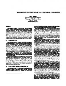
Table 2: Storage costs of four data structures on 3D data sets with non-manifold properties: Ent=#entities, Rel=#relations 8. Concluding Remarks We have addressed the issue of modeling non-manifold 3D shapes discretized as 3D simplicial complexes through a decomposition-based approach. To this aim, we have described a data structure for 3D simplicial complexes embedded into 3D Euclidean space based on unique and sound decomposition of such complexes into nearly manifold components, that we termed the DLD data structure. The structure of the decomposition is encoded as the upper level in the DLD data structure, while each nearly manifold component is described as an extended indexed data structure with adjacencies by encoding connectivity and adjacency relations. The DLD data structure is compact, since it explicitly encodes only vertices and top simplexes, it is highly scalable to the manifold case, and it supports efficient retrieval of topological relations. The DLD data structure is more expressive than the NMIA data structure [DH03], since it describes the non-manifold entities explicitly, and has almost the same storage cost. Also, navigation algorithms are simpler to implement on the DLD data structure since nonmanifold singularities are kept distinct from the lower-level representation of the IQM components. The DLD data structure, its construction and navigation algorithms have been implemented and tested on synthetic data sets. Figures 8(a)(f) show a 3D complex described by the DLD data structure.

(a)

(b)

(c)

(d)

(e)

(f)

Figure 8: (a) A wheel model with 1000 tetrahedra, 32 dangling faces and 96 wire edges; (b) a zoomed-in view of its center; (c) a side-way view; (d) the tetrahedral parts form three 3D manifold components; (e) the parts described by dangling faces form eight 2D components; and (f) the wire parts (enlarged)

A. Hui, L Vaczlavik and L. De Floriani / A Decomposition-based Representation for 3D Simplicial Complexes

A further important advantage of the DLD data structure is that it provides a unique decomposition of a 3D shape and thus is a very suitable basis for performing geometric reasoning of a 3D shape by identifying interesting topological features, and for shape understanding and recognition. The decomposition also makes it easier to extract topological invariants, such as Betti numbers, which can be used as a shape signature for reasoning and recognition purposes. 9. Acknowledgement This work has been partially supported by the European Network of Excellence AIM@SHAPE under contract number 506766, and by Project FIRB-MIUR SHALOM (SHape modeLing and reasOning: new Methods and tools) under contract number RBIN04HWR8 . References [CDM04] C UTLER B., D ORSEY J., M C M ILLAN L.: Simplification and improvement of tetrahedral models for simulation. In Proc. 2nd Eurographics SGP (2004). 1 [CKS98] C AMPAGNA S., KOBBELT L., S EIDEL H.-P.: Directed edges - a scalable representation for triangle meshes. J. of Graphics Tools 3, 4 (1998), 1–12. 3 [De 05] D E F LORIANI L.: Combinatorial characteristics of shapes. Lect. notes on Geometric and Solid Modeling (Fall 2005). Dept of Computer Science, Univ. of Maryland. 3 [DGH04] D E F LORIANI L., G REENFIELDBOYCE D., H UI A.: A data structure for non-manifold simplicial d-complexes. In Proc. 2nd Eurographics SGP (2004), ACM Press. 3, 8 [DH03] D E F LORIANI L., H UI A.: A scalable data structure for three-dimensional non-manifold objects. In Proc. 1st Eurographics SGP (2003), pp. 73–83. 2, 3, 8, 9 [DH05] D E F LORIANI L., H UI A.: Data structures for simplicial complexes: an analysis and a comparison. In Proc. 3rd Eurographics SGP (2005), pp. 119–128. 1, 3, 9 [DL89] D OBKIN D., L ASZLO M.: Primitives for the manipulation of three-dimensional subdivisions. Algorithmica 5, 4 (1989), 3–32. 3 [DMMP03] D E F LORIANI L., M ESMOUDI M. M., M ORANDO F., P UPPO E.: Non-manifold decompositions in arbitrary dimensions. CVGIP: Graphical Models 65, 1/3 (2003), 2–22. 1, 3, 4, 6 [DMP03] D E F LORIANI L., M ORANDO F., P UPPO E.: Representation of non-manifold objects in arbitrary dimension through decomposition into nearly manifold parts. In 8th ACM Symposium on Solid Modeling and Applications (June 2003), ACM Press, pp. 103–112. 4 [DMPS04]

D E F LORIANI L., M AGILLO P., P UPPO E., S O BRERO D.: A multi-resolution topological representation for non-manifold meshes. Computer-Aided Design J. 36, 2 (February 2004), 141–159. 3

[Ede87] E DELSBRUNNER H.: Algorithms in Combinatorial Geometry. Springer Verlag, Berlin, 1987. 3, 8 [FR92] FALCIDIENO B., R ATTO O.: Two-manifold celldecomposition of R-sets. In Proc. Computer Graphics Forum (1992), vol. 11, pp. 391–404. 3 [FRL00] F INE L., R EMONDINI L., L ÉON J.-C.: Automated generation of FEA models through idealization operators. Int’l J. for Numerical Methods in Engineering 49 (2000), 83–108. 1 [GTLH98] G UEZIEC A., TAUBIN G., L AZARUS F., H ORN W.: Converting sets of polygons to manifold surfaces by cutting and stitching. In Conference abstracts and applications: SIGGRAPH 98 (1998), ACM Press, pp. 245–245. 3 [LL01] L EE S. H., L EE K.: Partial-entity structure: a fast and compact non-manifold boundary representation based on partial topological entities. In Proc. 6th ACM Solid Modeling and App. (2001), ACM Press, pp. 159–170. 3 [LNPT00] L OPES H., N ONATO L. G., P ESCO S., TAVARES G.: Dealing with topological singularities in volumetric reconstruction. In Curve and Surface Design (2000), Vanderbilt University Press, pp. 229–238. 3 [LT97] L OPES H., TAVARES G.: Structural operators for modeling 3-manifolds. In Proc. 4th ACM Solid Modeling and App. (1997), ACM Press, pp. 10–18. 3 [MH01] M C M AINS S., H ELLERSTEIN C. S. J.: Out-of-core building of a topological data structure from a polygon soup. In Proc. 6th ACM Solid Modeling and App. (2001), pp. 171–182. 3 [Muc93] M UCKE E.: Shapes and Implementations in ThreeDimensional Geometry. PhD thesis, Dept of Computer Sci., Univ. of Illinois at Urbana-Champaign, Urbana, 1993. 3 [Nab96] NABUTOVSKY A.: Geometry of the space of triangulations of a compact manifold. Commun. Math. Phys. 181 (1996), 303–330. 4 [Nie97] N IELSON G. M.: Tools for triangulations and tetrahedralizations and constructing functions defined over them. In Scientific Visualization: overviews, Methodologies and Techniques. IEEE Computer Society, 1997, ch. 20, pp. 429–525. 3, 7 [PTL04] P ESCO S., TAVARES G., L OPES H.: A stratification approach for modeling two-dimensional cell complexes. Computers and Graphics 28 (2004), 235–247. 3 [RO90] ROSSIGNAC J. R., O’C ONNOR M. A.: SGC: a dimension-independent model for point-sets with internal structures and incomplete boundaries. In Geometric Modeling for Product Engineering. Elsevier Sci. Publishers B. V., 1990, pp. 145–180. 3 [VL97] V ÉRON P., L ÉON J. C.: Static polyhedron simplification using error measurements. Computer-Aided Design 29, 4 (1997), 287–298. 3 [Wei88] W EILER K.: The radial-edge data structure: a topological representation for non-manifold geometric boundary modeling. In Geometric Modeling for CAD Applications. Elsevier Sci. Publishers B. V., 1988, pp. 3–36. 3

[DS92] D ESAULNIER H., S TEWART N.: An extension of manifold boundary representation to R-sets. ACM Trans. on Graphics 11, 1 (1992), 40–60. 3 c The Eurographics Association 2006.