A Distributed Agent-based Simulation Environment for ... - CiteSeerX

Accepted to Special Issue on Software Agents and Simulation, SIMULATION, April 2001

A Distributed Agent-based Simulation Environment for Interference Detection and Resolution * S. Ramaswamy Software Automation and Intelligence Laboratory Computer Science Department Tennessee Technological University Cookeville TN 38505 Email: [email protected]

K. Srinivasan, P. K. Rajan, S. Krishnamurthy Electrical and Computer Engineering Department Tennessee Technological University Cookeville TN 38505 Email: [email protected]

In this paper, a two-level architecture is developed and implemented for the interactive simulation and evaluation of a distributed agent-based simulation environment designed to detect and resolve interference in naval radar units. The Java-based simulation is designed as a two level software architecture incorporating: i) multiple radars on each ship controlled through a lower-level intra-ship interference control module, and, ii) multiple ships in a group coordinated through a higher-level interference control module. Each ship’s interference detection and resolution mechanism, termed a control agent, is composed of these two separate levels, which dynamically coordinate to detect and then resolve interference problems using three different coordination strategies - a Master-Slave, a Locally Autonomous and a simple Negotiation mode.

*

R. MacFadzean Naval Surface Warfare Center Dalhgren, Virginia Email: [email protected]

1. Introduction Currently the US Navy uses a personal computer based program called the Electromagnetic Compatibility Analysis Program (EMCAP) to develop plans for controlling radar interference. These plans may be for a single platform or a battle group, and can include frequency changes, position changes, and radar mode changes. One ship serves as a central frequency manager (CFM) that sends messages to each ship requesting it to return the desired frequencies for each of its radar units. Each ship independently determines the desired operating parameters for each radar unit, formats a message, and forwards it to the CFM. The CFM then analyzes the frequency requests considering the relative positioning of the ships and determines whether ships will have interference for their chosen frequencies. If they are going to have interference, then the CFM assigns a new frequency to one or all ships in order to avoid interference. Under some conditions, position changes or radar mode changes may also be assigned. Each ship is equipped with an EMCAP computer, with one ship/system designated the CFM. The system does not perform real-time coordination and has human elements in the loop that causes considerable delays. The process can take hours. It is possible that a distributed approach to interference management would pay benefits in terms

This research is currently being conducted at the Software Automation and Intelligence Laboratory (SAIL) in the Computer Science Department at Tennessee Technological University and was supported, in part, by grants from the National Science Foundation (#DMI 9896235) and the Center for Manufacturing Research at Tennessee Technological University.

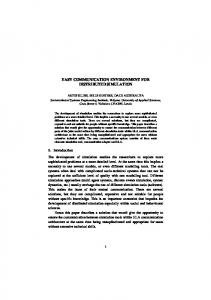
of timeliness and effectiveness, but testing would be very expensive. Prototyping new concepts for naval radar frequency assignment in a distributed simulation environment is an excellent way to test and evaluate new hardware, software, and algorithms in a system level configuration. In this paper, the development of a two-level distributed agent-based interactive simulation environment for the implementation and evaluation of the above mentioned interference detection and resolution problem is presented. Also, the paper addresses the implementation and evaluation of different coordination strategies for interference resolution. The two-level architecture, as shown in Figure 1, consists of a lower level and a higher-level control module. While the lower level module resolves the interference problem between radar units on the same ship, the higher level module handles the responsibility of resolving interferences between radar units on multiple ships in the group. The higher level module first detects the (outside) source of interference. If the source is a radar unit on another ship within the group, it may resolve the interference problem in one of the following three modes, viz. Master-Slave, Locally Autonomous, or the Negotiation-based mode. The approach provides the following advantages. 1. The two-level approach helps in balancing between local and system goals and in developing appropriate data structures and encapsulation techniques for addressing such concerns appropriately. Here the local goal of every ship is to provide interference free operating frequencies to its radar units and the system goal is to provide interference-free operating frequencies for all radar units on all the ships within the group. 2. Using the proposed architecture, it is easy to implement and study algorithms for group coordination. Different coordination and group management (arbitration, election of a group representative, determining group membership eligibility, rescinding / retaining group memberships, etc.) algorithms may be selectively implemented and evaluated. 3. The two-level structure incorporates a separate database associated with every ship. By creating a separate thread of control for coordinating (i.e. reporting and maintenance) database related information to legal group members, the simulation provides for any ship to assume control. 4. The two-level implementation provides a generic test-bed for studying various performance issues. These include available reaction time with respect to the speed of interference detection and its

2

DATABASE

Control Agent

GLOBAL

LOCAL

HIGH LEVEL

Resolving Inter-Radar Interference between Different Ships

Database Handler

LOW LEVEL

Resolution of Intra-Radar Interference within the Same Ship

RADAR 1

RADAR 2

RADAR 3

RADAR 4

-----

RADAR N

Figure 1. Two-level Control Agent Architecture

subsequent resolution; estimation of the percentage of false alarms (Note: effects of false alarms are not investigated in this paper) and the consequences of subsequent actions; etc. Interference for a given radar may be due to either of the following three reasons: i) another radar in the same ship, ii) radar of another ship in the same group, or iii) an external interference. In this paper the first two cases are referred to as intra-ship interference and inter-ship interference, respectively. In reality, such interference problems can be resolved by either changing the radar’s frequency, bandwidth or position [1]. However, it is desirable to change a radar unit’s frequency to resolve interference. Therefore, this simulation environment focuses on quickly identifying and switching to a frequency that eliminates such interference. The two-level distributed simulation architecture for radar frequency assignment is implemented using software agent techniques. An agent-based implementation provides an ideal basis for implementing and evaluating various communication strategies. In general a software agent is defined as a program/module that has some level of autonomy, cooperation and learning capabilities. In this application each ship is implemented as a software agent to form a multi-agent system (MAS). The ships (or agents) interact with each other in any of the three coordination modes to choose interference free frequencies for their respective radar units. Conceptually, a software agent helps inter-operability between programs wherein these agents communicate with each other using some agent communication language in order to provide services that cannot be rendered if the programs were to execute in a standalone mode. In [2], the definition of an agent by IBM, is stated as: “Intelligent agents are software entities that carry out some set of operations on behalf of the user or another program with some degree of

independence or autonomy, and in so doing, employ some knowledge or representation of the user’s goals or desires.” The authors also state that, in actuality, an agent represents two orthogonal concepts, which are, (i) the agent’s ability for autonomous execution, and (ii) the agent’s ability to perform domain oriented reasoning. In this paper, we will define an agent to be a software module that exhibits the above mentioned orthogonal concepts. To attain a high level of interoperability between software systems on multiple platforms, knowledge of each other's capabilities is required, for tasks such as planning, monitoring and resource allocation to be easily accomplished. Software agents have been classified as the following [3-6]: Collaborative, Interface, Mobile, Information or Internet, Reactive, Hybrid and Smart agents. Similar to

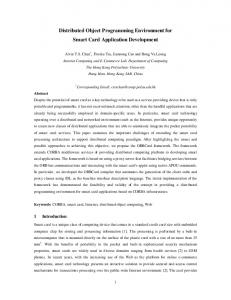
dynamically coordinates with other such control agents, as shown in Figure 3, in eliminating interference problems. In addition, each control agent is designed to execute as a multi-threaded process incorporating a periodically updated database containing information about radar units on the ship and within the group. The database is designed to provide complete information about all the radar units on every ship in the group. As stated earlier, each control agent is a two-level architecture consisting of the lower and higher-level modules. Each CA is also designed to coordinate using three different coordination modes with other such agents. These CA Server of Ship

CA Server of Ship

begin Start-up

Initialization run

Halt

Reset and restart

Execute

CA Server of Ship

CA Server of Ship

complete

Figure 2. A Simple Agent Lifecycle

applets, agents also have well-defined lifecycles [7, 8]. Figure 2 illustrates the four different states that make up an agent lifecycle [7]. Agents have been used in a variety of applications. Examples include MIT Media laboratory's user interface for IRC(Internet Relay Chat) [9] called the “Butterfly Agent”, space operations [10], image analysis [11], power applications [12] , simulation [13- 14], adaptive behavior of humans in hazardous / critical environments such as nuclear plant, satellite ground system or an industrial control system [15]. The above survey is a brief introduction into some recent agent-based implementations of simulation applications. For a detailed introduction on agents, their definitions, capabilities, and other applications, the reader is referred to [16-25] and references therein. For the radar interference model used in this paper for the detection and resolution of interference, the interested reader is referred to [1, 26-28]. The rest of this paper is organized as follows. Section 2 describes the system architecture and the associated database. Section 3 provides a brief review of the implementation and Section 4 provides the results of the comparative simulation and evaluation of the three different coordination strategies and Section 5 presents a summary of the results obtained. Section 6 concludes the paper.

2. The Control Agent Architecture Each ship's interference detection and control mechanism is composed of two separate levels, henceforth, referred to as a control agent (CA), which

3

Figure 3. Control Agent-based Structure

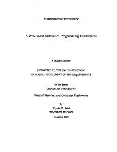
coordination methods include i) Master-Slave mode: In the master-slave mode, control is strictly hierarchical and top-down in nature using a table look-up technique. ii) Locally Autonomous Mode: In this mode, decisions are always made locally and based upon local goals of the agent without regard to the overall system goals. iii) Negotiation based mode: In this mode, the resolution of any potential conflicts is always through negotiation between the processes that experience the conflict, possibly with the aid of an arbitrator. At the lower level, the control agent resolves potential interference problems either through a master-slave or locally autonomous mode. At the higher-level, the control agent may adopt any of the three techniques. At the lower level, the control agent monitors and logs information about its radar units continuously. If the server finds that a radar unit is experiencing interference, and determines that the interference is local, i.e., caused by some radar within the ship, then in such a case, it assumes the responsibility of reassigning a frequency to either the interfering radar or both the radar units. As shown in the class diagram of Figure 4, the lower level control agent has complete access to the radar information about radar unit in the current ship from the database. Alternatively, if a radar unit within the ship does not cause the interference, then the control is transferred to the higher-level control agent. This is because the lower level control agent cannot communicate with other ships in the group and hence

will not be able to modify the database with information pertaining to radar units on other ships. The higher-level module has complete access to the portion of the database that contains information about radar units on other ships. The higher level of the control agent can operate in any one of the following modes: MasterSlave, Locally Autonomous or the Negotiation based mode. In the Master-Slave mode the higher level cooperates and accepts decisions made by the group coordinator. Whenever it encounters an external interference it makes a request to the group coordinator that acts as a master control agent, for a new frequency. The master control agent may either allocate a new set of frequencies to all the radar units on the ship that are experiencing interference, or assign a new frequency to individual radar. In a locally Figure 4. Lower-Level Control Agent Class Structure autonomous mode, the higher level module in each ship does sources, i) information about the local radar units and not communicate with other ships in the group to ii) information about the group’s radar units (i.e., radar resolve its interference, but does signal to the rest of units on other ships). The local information in the the group on any changes that it makes to its radar database can be updated by lower level of the control frequencies. Thus each ship may resolve its agent. The lower level control agent does not have the interference problem by randomly switching to a new ability to modify the information about radar units on frequency whenever it faces inter-ship interference other ships within the group. This information can be problems. In a negotiation-based mode, each ship tries accessed and updated only by the higher-level control to identify the source of the interference. If the source agent. Whenever a radar unit information is updated on is one of the members of its own group, it sends a a ship, the handler broadcasts this information to the message to the ship seeking a negotiation. When the control agents on all ships. The control flow within the ship causing the interference acknowledges the database is illustrated in Figure 5. message, the two ships negotiate and settle for a 2.2. The lower-level Control Agent frequency that is ideal for both of them. This system The class hierarchy of the lower level control agent, has a real-time co-ordination unlike the central Ship

Constants

$ pi: float=(float) 3.14159 $ k:double=1.38E-23 $ fourpi_squared:(float) 157.9 $ fourpi_cubed:float=(float)1984.4 $ fourpi_squared_db:float=(float)21.98 $ fourpi_cubed_db:float=(float)32.98 $ c: float=30000000 $ DUCT: float=30 $ Gmutual_db:float=7 $ Gantenna_db:float=7 $ FofrMIN_db:float=-130 $FofrMIN: double= 1.0E-13

info

DB

s

+map

radarList: Vector shipList: Vector

ShipCanvas

ShipImage

s: ShipInfo Radars[]: RadarImage ShipImage()

RadarImage

Interference Points

state: int r:Radar tt:LwToolTips

LwToolTips

message: String fm: FontMetrics

RadarImage() paint()

LwToolTips() LwToolTips() set() paint()

+r

Radar

Formulae

log() dBValueOf() square() distance() distance() ThermoNoise() Fprop() Fofr() SignalLvOf1At2() SigStrOfTargAtRadr() main()

x:float y:float z:float speed: float losses: float address: int

Database

Database() setRadarList() setShipList() updateRadar() updateShip() getRadar() getShip() addRadar() addShip() delRadar() delShip()

ShipName1: String ShipName2: String RadarName1: String RadarName2: String

ShipInfo

Ship() Main() autonomous() Interference Detection Algorithm() paint()

RadarInfoDlg

radarFreq :Textfield radarPower:Textfield radarAntGain:Textfield radarHorizWidth:Textfield radarVertWidth:Textfield radarAntRotateRate:Textfield radarPulse:Textfield radarTemp:Textfield radarName:Textfield thisRadar: Radar Ok: Button Cancel: Button

thisRadar

freq: float peakPower: float maxAntGain: float horizBeamWidth: float vertBeamWidth: float antRotateRate: float pulseWidth: float temperature: float state: int block: boolean shipName: String radarName: String

RadarInfoDlg() getRadar() setRadar() actionPerformed()

frequency manager. Conceptually, the control agent implementation is split into three distinct processes. These include i) The database system, ii) The lower level control agent iii) the higher level control agent. In the remainder of this section, we will discuss each of these processes in detail. 2.1. The Database Each ship has a database (server) that runs in an infinite loop, which can connect to the lower or higher level of the control agent through a database handler. The database consists of two distinct information

4

public void run() { try { // Socket ready for connecting lower/higher level of control agent // Accept connection // Open Output Stream to send data to control agent // Open Input Stream to read data from control agent // String lower/higher level of control agent // String code from control agent for local or global access by higher/lower // level of control agent // Make sure everything is cleanly connected // Lower/Higher level of control agent reads data from local/global database respectively // Lower/Higher level may write into the local/global database respectively // Close connection } catch(IOException e) { } }

Figure 5. Control Flow within the Database Handler

radar interference resolution class handles interference problems referred to by the lower-level control agent. First using its current database information, it tries to identify the source ship and then initiates a communication with the control agent.

Control-Agent Coordinator

Multiple threads connecting other Control Agents

Control-Agent Process Connection Process Process

Database (Local and All Ships)

Inter-radar Interference Resolution Algorithm

Local Ship

Other Ships Process Process Process

Figure 6. Higher Level Control Agent Class Structure

i.e., the Ship class, is shown Figure 4. The Database class is used to update and maintain the information about all the radar units on the ship. The options that are available in this class are shown clearly in the class diagram. Radar units can be added or removed from the ship and this class updates their operating parameters and position. The Ship class can read, write or update local information into the database only and does not have access to modify the global information within the database. 2.3. The Higher-level Control Agent The higher-level control agent does frequency resolution involving radar units on multiple ships. The control-agent runs in an infinite loop with a socket ready to accept a communication from any other group member. When a new control agent (ship) enters the group it sends an identifier to the coordinator for authorization. After authorization the client has to send all its parameters. The client information is registered by the coordinator and broadcast to the rest of the group only if it sends all its operating parameters to the coordinator after authorization. If two clients try to connect at the same time, then the client that sends its complete message first gets registered, while the other client has to try and connect again, possibly with a different id if necessary. The simulation is executed as a client/server application. If a ship that serves as a coordinator is destroyed / loses communication with the rest of the group, then another ship is dynamically voted to be a coordinator. The current coordinator may be referred to as the active coordinator while all other ships can be thought of as passive coordinators. The schematic of the higher-level control agent is shown in Figure 6. The control agent class is a multithreaded implementation consisting of the controlagent connection, database, inter-radar interference resolution and the ship classes. The control-agent connection class initiates multiple socket connections to other members of the group for interference resolution. The database class has the complete list of all the radar units on the ship and about the radar units on all other ships. The higher-level control agent maintains and updates all database entries. The inter-

5

3. Implementation Details A major objective of the implementation is the robust assignment of interference free frequencies (after a detection) to radar units in all ships in a distributed simulation environment. KQML (Knowledge Query Manipulation Language), a protocol developed by ARPA for supporting interaction and communication between intelligent software agents, is used for communication between higher-level control agents. The implementation includes (i) Control Agent, (ii) Database (iii) Inter-radar Interference Resolution Algorithm and (iv) Ship classes. Each of the individual classes is discussed in detail in the following subsections. Figure 7 is a simple schematic representation of how control agents use the KQML protocol for communication. When a control agent composes a message it goes to the KQML Layer, where the message content gets wrapped into a KQML message. The KQML protocol does not know anything about the message but for the beginning and end of the message. Thus the KQML message is sent to the other control agent. At the receiving end the KQML Layer parses the message and extracts the contents of the message and passes it to the control agent. A KQML code in which a control agent starts a conversation with another control agent is given in Control Agent

Control Agent

Message

Message

KQML Layer

KQML Layer

KQML Message

KQML Message

Internet

Figure 7. KQML Based Interaction (ask-one : content ( “HELO”) : receiver control agent B : language KQML : ontology NEGO)

(reply : content ( “HELO”) : receiver control agent A : language KQML : ontology NEGO)

Ask-one: S wants an answer from R.

reply: R is sending a reply for S’s Query.

Figure 8. A KQML Structure

Control Agent 1 (Master)

Control Agent 2 (Slave) Slave Watcher

starts

Slave Watcher Slave Listener

Slave Listener Master

starts

starts

starts

Master Thread

Control Agent 1

Control Agent 2 Slave Watcher

starts

Slave Watcher Slave Listener Connects

starts

starts

starts

starts

starts Interfering frequency

starts

destroy

destroy

IDRL_NE

IDRL_MS

IDRL_MS

starts

Slave Listener

Slave Listener Thread

Interference Detection every 6 seconds


starts

starts

IDRL_NE Interference Detection every 6 seconds


starts

Connecting to Master sendINTR() Interference free free frequency (f)

sendUPRD()

Figure 9. Interaction diagram in the Master-Slave Mode

Figure 8. Basically a KQML message consists of a performative and associated arguments that includes the actual message content. The performative is used to specify whether the message in the content field is a command, assertion or a query. Here the message content is “HELO” i.e. control agent A is starting conversation with control agent B. “ask-one” and “reply” are the performatives used by the Sender (S) and Receiver (R) respectively. The other arguments receiver, language and ontology are used to specify as to which control agent the message is intended to, the language used and the context respectively. More information on KQML can be found in [29-32]. 3.1. Higher-level Control Agent The schematic of the implementation of the higherlevel control agent is given in Figure 6. All control agents in the group run in an infinite loop ready to accept client connections from another ship. Whenever a ship joins or leaves a group or whenever a radar is added or removed from a ship, the information is broadcast to all the ships in the group. The Database class is used to hold all the ship and radar information of all ships in the group. Each ship can connect to its database and access information from it. The database consists of two distinct information sources, i) information about the local radar units and ii) information about the group’s radar units. The higher-level control agent has Figure 10. Interaction access to the entire diagram in a Locally database. Error autonomous mode Control Agent 1

Slave Watcher

starts

Slave Listener

send UPRD()

Interference free frequency (f)

Figure 11. Interaction diagram for Negotiation mode

messages are displayed whenever wrong values of variables are entered in the ship and radar information dialogue boxes. Table 1 provides some sample radar parameters used in the simulation. As stated earlier, the control agent can be started in three different modes for coordination and communication; viz: Master Slave, Locally Autonomous and Negotiation. The interaction diagrams [33] for these modes are illustrated in Figure 9, Figure 10, Figure 12. Radar properties and Figure 11. A interface screenshot of the radar information dialogue box is shown in Figure 12 and a screenshot of the implementation of the lower level control agent (ships) is shown in Figure 13.

4. Performance Evaluation

starts

IDRL_LA

starts

sendUPRD()

6


Interference free frequency (f)

In order to evaluate the efficiency of each of the three modes namely the locally autonomous, master-slave and negotiation modes, an identical test code was plugged into each of these modules individually. The module recorded interference detection and resolution times by any of the ships in the group. Interference was created between ships by manual entry between two or more ships having two or more radars on each ship. Whenever interference was detected by any of the ships within the group, the time at which the interference was detected was written into a report file using a file output stream by the test module. Similarly

the time at which interference was resolved was also logged into the report file. Appropriate graphs were plotted for the test results. The testing was divided into four distinct cases. These different cases are described below with the accompanying results in the form of graphical plots between the number of ships within the group and the time it took to resolve interference. Note that the time it took to subsequently update the database on every ship is left out so that we look into the actual time involved in interference resolution irrespective of the network delays and other database related synchronization issues, etc. Figure 13. Lower level control agent interface 4.1. Experimental set up and assumptions separation required for a bandwidth of 1.2 MHz. For The following assumptions were made in the example, two radar units with 0.4 MHz bandwidths simulation. (i) All control agents are simulated on a require a minimum frequency Separation of 1 MHz to Windows NT machine with one control agent/ship. (ii) operate without interfering with each other. Similarly, The number of ships in a group varied from two to ten. 0.6, 1.2, 2.4, and 5 MHz radar units require a minimum (iii) The number of radars in every ship varied from frequency separation of 2, 3, 5,and 10 MHz, one to five. (iv) All tabulations in the four cases show respectively for interference- free operation. Hence the time for interference resolution in milliseconds suitable frequency ranges were chosen appropriate to while on the three different modes of interaction. The each case. graphs are plotted against the number of radars and Figure 14 - Figure 22 provide the graphical plots for time for interference resolution. all these three sub-cases. It can be seen that the Assumptions about the radar units include the negotiation-based approach takes less time for following (i) All radar units in all the ships in the group resolving any interference. have the same receiver threshold power of –70 dB. (ii) Case II: Homogeneous Bandwidths within a Ship All radar units in all the ships in the group have the same peak transmitting power of 200 kilowatts. (iii) In In this case, all radar units on a given ship operated all the test cases a moderate ducting factor is used on the same bandwidth and radar units in other ships while calculating the propagation factor. had bandwidths that were homogeneous within the ship, yet different from other ships in the group. Figure Case I: Homogeneous Bandwidths across the Group: 23 - Figure 25 provide the plots for this case and it can In this case, all the radar units in all the ships in the be seen as in Case I that a negotiation based approach group are assumed to operate with the same bandwidth, i.e. similar operating Table 1: Typical Radar Parameters bandwidths were chosen Radar Parameter Description for all radars on all ships. Radar id Unique Identifier for each radar in the simulation process This case was divided into Peak Power (P) 250000 to 500000 watts (54 to 57 dB w) three sub cases based on Maximum Antenna Gain (G) 200 to 300 (23 to 24.8 dB) the bandwidths chosen for Wave length (λ) .230 to .224 meters - λ= c/f, where c= speed of light (300 the simulation. Case IA m/µs) and IB: All radar units on (λ2 =. 0529 to .0502 m2, -12.77 to -13.00 dB meters) all ships had a bandwidth Frequency (f) 1300 to 1340 MHz Losses (L) .80 to .50 (-1 to -3 dB) of 0.4MHz and .6 MHz .50 to 2.0 ms Pulse width (τ) respectively, with a Pulse Repetition Rate (prf) 800 to 2500 pulses/second frequency range of 1300Antenna Hor. Beam width 4 degrees 1400 MHz. Case IC: All (thh) radar units on all ships Antenna Vert. Beam width 15 degrees have bandwidth of 1.2 (thv) MHz. with a frequency Antenna Rotating Rate (thdot) 180 degrees/second range of 1300-1450 MHz. System Temperature (Ts) 900 to 1100 K The differences in Easting Position (x) -100000 meters to +100000 meters frequency ranges were Northing Position (y) -100000 meters to +100000 meters necessary to enable the Antenna Height (z) 20 to 30 meters minimum frequency State Interference free, Interfering with another radar or shot.

7

separation required between radar units in order to avoid interference was 10 MHz. To theoretically fit 40 units, the frequency range required was 1300 to 1700 MHz. In both cases IVA and IVB, it was found that using all the three possible approaches used for interference detection, each approach fit 37 out of 40 possible radar units. Thus, the algorithms were found to be 92.5% efficient in finding interference free frequencies for the radar units with interference.

provided the most efficient solution. Case III: Heterogeneous Bandwidths within a Ship In this case, all radar units on a given ship operated on different bandwidths and radar units in other ships also had different bandwidths between their radars. Figure 26 - Figure 28 provide the plots for this case and it can be seen as in Cases I and II, the negotiation based approach provides the best possible solution with the least time required to resolve interference problems. 4.2. Case IV In this case, the efficiency in finding an interferencefree operating frequency in each mode was measured by overloading the algorithms given a narrow frequency range for operation and introducing as many radar units as possible within this range. Then they were compared against a theoretically optimal solution. This case has two sub-cases, IVA and IVB. In case IVA all radar units in all the ships were instantiated with the same peak power and threshold, and the bandwidth was set to 2.4 MHz. Thus the minimum frequency separation required between radar units to avoid interference was 5MHz with a frequency range is 1300 to 1500 MHz. Theoretically 40 different radar units can be "fitted" within this range. In Case IVB all radar units had a bandwidth of 5 MHz bandwidths. Thus the minimum frequency

5. Results and Analysis In all the above simulation experiments, it was found that when the number of ships was less than five, all the modes performed equally well. As the number of ships and the number of radar units per ship increased, the time taken by the negotiation-based approach proved to be invariant compared to the master-slave and locally autonomous modes. In fact both the Master-slave and locally autonomous modes showed a rapid increase in the time required for interference resolution with increased load. One possible reason for the negotiation-based approach to outperform the locally autonomous mode may be because in the locally autonomous mode, the affected ship changes to a new random frequency without checking with the existing frequencies. That is, the

Case 1B: Locally Autonomous Mode

10000 5000

15000.00 10000.00

Case IC: Locally Autonomous Mode

5000.00 0.00 2

0 2

3 4 5 6 7 8 Number of Ships (Max: 10057, Min 223)

9

3

4

5

6

7

8

9

10

Number of Ships (Max: 12055, Min 212)

10

Time to Resolve Interference (ms)



Case 1A: Locally Autonomous Mode

15000.00 10000.00 5000.00 0.00 1

2

3

4

5

6

7

8

9


Figure 14. Interference Resolution Time Plot: Case IA - All Radars with 0.4 MHz Bandwidths

Figure 17. Interference Resolution Time Plot: Case IB - All Radars with 0.6 MHz Bandwidths Case 1B: Master Slave Mode

Figure 20. Interference Resolution Time Plot: Case IC - All Radars with 1.2 MHz Bandwidths

10000 5000

15000.00

Case IC: Master Slave Mode

10000.00 5000.00 0.00 2

0 1

2 3 4 5 6 7 Number of Ships (Max: 1381, Min 342)

8

3

4

5

6

7

8

9

10


9




Case 1A: Master Slave Mode

15000.00 10000.00 5000.00 0.00 2

3

4

5

6

7

8

9

10



Figure 18. Interference Resolution Time Plot: Case IB - All Radar Units with 0.6 MHz Bandwidths


Case 1B: Negotiation Mode

Case IC: Negotiation Mode

10000 5000 0

15000.00 10000.00 5000.00 0.00 2

2

3

4 5 6 7 8 Number of Ships (Max: 381, Min 467)

9

10


8

3

4

5

6

7

8

9

10


Figure 19. Interference Resolution Time Plot: Case IB - All radars with 0.6 MHz Bandwidths




Case 1A: Negotiation Mode

15000.00 10000.00 5000.00 0.00 2

3

4

5

6

7

8

9

10



goal of providing interference free operating frequencies to radar units on a given ship is uniquely addressed by the lower level module, the higher level module maintains responsibility for issues such as inter-group communication and coordination, and database consistency. In its current form of the simulation, the group coordinator and all other ships operate on the same mode of communication. The possibility of different ships using different coordination schemes based on the systems load, history and other such parameters is being investigated.

locally autonomous mode favored a quick resolution in achieving a local goal of providing interference-free frequencies to its local radars (i.e. in a single ship), and not taking into consideration interference issues with all radar units (i.e. in all of the ships). Therefore, as the number of ships increased, these solutions created interference with existing radar frequencies on other ships. In the master-slave mode, the designated master ship provided client ships with possible interference-free frequencies after checking its database. However, when the number of ships increased, the communication load on the master ship became high due to the handling of multiple client requests at the same time. Thus as the number of ships and the number of radars per ship increased, the algorithm started performing poorly. The existing interference detection algorithm continuously checks for the interference every six seconds. A modified version designed using a try-catch interrupt routine was implemented and it was observed that the performance results were not affected by such a implementation for this case study. However, it is our view that, such a implementation may provide a better execution performance for some domains.

6. Conclusions

9

The authors would like to thank Joe Cherry, Thad Scalf, Dr. Roger Haggard and Dr. Jeff Frolik, of the ECE department at Tennessee Tech. for their help in the design and presentation of this work.

8. References 1. R. Macfadzean, S. Ramaswamy and K. S. Barber, "Radar Frequency Assignment in Mobile Radar Units", Workshop on Semiotic Modeling for Case III: Locally Autonomous Mode

Case II: Locally Autonomous Mode



20000.00 15000.00 10000.00 5000.00 0.00 2

3

4

5

6

7

8

9

20000.00 15000.00 10000.00 5000.00 0.00 2

10

3

Figure 23. Interference Resolution Time Plot: Case II - Homogeneous Distribution - All Radars on Same Ship with Same Bandwidths



10000.00 5000.00 0.00 3

4

5

6

7

8

5000.00 0.00 2

3

4

5

6

7

8

9

10

Figure 27. Interference Resolution Time Plot: Case III - Heterogeneous Distribution - All Radars on Same Ship with different Bandwidths Case III: Negotiation Mode


15000.00 10000.00 5000.00 0.00 6

10

10000.00

Case II: Negotation Mode

5

9

Number of Ships (Max: 5735, Min: 355)

20000.00

4

8

15000.00

9


3

7

20000.00

Number of S hips (Max:5628, Min 345)

2

6

Case III: Master Slave Mode

15000.00

2

5

Figure 26. Interference Resolution Time Plot: Case III - Heterogeneous Distribution - All Radars on Same Ship with different Bandwidths

Case II: Master Slave Mode

20000.00

1

4




In this paper, a two-level agentbased, simulation architecture for interference resolution between ships with multiple radar units has been presented. Also, three different communication and coordination modes between these radar units have been evaluated. The main advantages of having such an architecture are the following. (i) Identifying and estimating the time to resolve interference is useful in devising appropriate interference resolution schemes to provide accurate data for logistics and planning activities. (ii) Maintaining a periodically updated database containing information about radar units on all ships within a group is useful in localizing much of the decisions made and hence reducing network traffic. This also helps in localized planning. (iii) The twolevel simulation architecture helps in understanding the implications of the delicate tradeoff mechanisms between addressing the requirements related to local and system goals. While the local

7. Acknowledgements

7

8

9

10

Number of Ships (Max:468, Min 382)


20000.00 15000.00 10000.00 5000.00 0.00 2

3

4

5

6

7

8

9

10


Figure 28. Interference Resolution Time Plot: Case III - Heterogeneous Distribution - All Radars on Same Ship with different Bandwidths

Sensible Agents, Intelligent Systems: A Semiotic Perspective, NIST, Gaithersberg, MD, Oct. 1996. 2. Stan Franklin and Art Graesser, “Is it an agent, or just a program? A Taxonomy for Autonomous Agents”, http://www.msci.memphis.edu/~franklin/AgentProg .html (current: 8/10/2000) 3. T. Kurki, “Internet Agents”, http://smartpush.cs.hut.fi/SoftwareAgent…pers/Inte rnet_Agents/Internet_Agents.html (current: 8/10/200) 4. J. Bradshaw “An Introduction to Software Agents”, http://www.cs.umbc.edu/agents/introduction/01Bradshaw.pdf (current: 8/10/2000) 5. Hyacinth S. Nwana and Divine T. Ndumu “A Perspective on Software Agents Research”, http://www.cs.umbc.edu/agents/introduction/hn-dnker99.html (current: 8/10/2000) 6. K.S. Barber, T.H. Liu, A. Goel, S. Ramaswamy, “Flexible Reasoning using Sensible Agent-based systems: A case study in job-flow scheduling”, Intnl. Jour. of Prod. Plan. & Ctrl., Vol 10, No. 7, 1999, pp. 606-615. 7. R. Chakrapani, “Mobile Agents: An Overview”, Graduate Seminar, Georgia Southwestern University, Unpublished report. 8. T. Sundsted, "Agents on the move: Bolster your client apps by adding agent mobility", http://www.javaworld.com/javaworld/jw-071998/jw-07-howto.html 9. N. W. Van Dyke, H. Lieberman, P. Maes, “Butterfly: A Conversation Finding Agent for Internet Relay Chat” http://www.media.mit.edu/~nwv/projects/butterfly (current as of 8/10/2000) 10.S. Mandutianu, A. Stoica, “An Evolvable MultiAgent System for Space Operations Engineering”, Intn. Conf. on AI, Las Vegas, NV July 1999. 11.The Agent-based, Automatic Parallelization of Image Analysis Tasks Project, http://www9.in.tum.de/research/parallel/ (current as of 8/10/2000) 12.R. Gustavsson, “Agents with Power”, Comm. of the ACM, Vol. 42, No. 3, March 1999 13.A. Chan, Tim Spracklen, "Web-Based Distributed Object Simulation Framework", SCSC 99, Chicago, IL, pp.9-13 14.G. Pitts, S. P. Hwang, "An intelligent interface agent: Simulation/Modeling made simple", SCSC 99, Chicago, IL, pp: 103–105. 15.N. R. Edala, M. Garay, S.Narayanan, "A Distributed simulation environment for analyzing adaptive agent behavior in supervisory control systems", ", SCSC 99, Chicago, IL.

10

16.S. Jernigan, S. Ramaswamy, K. S. Barber, “A Distributed Search and Simulation Method for Job Flow Scheduling”, SIMULATION, June 1997. 17.J. Rosenschein, “Rational Interaction: Cooperation Among Intelligent Agents”, Ph. D. Thesis, Technical Report # STA-CS-85-1081, Stanford University, 1986. 18.S. Kraus, J. Wilkenfeld, “Negotiation over Time in a Multi Agent Environment”, Technical Report UMIACS-TR-91-51, University of Maryland, Institute of Advanced Computer Studies, 1991. 19.J. Doyle, “Rationality and its Roles in Reasoning”, Comp. Intel., Vol. 8, No. 2, pp. 376-409, 1992. 20.Y. Shoham, “Agent-Oriented Programming”, AI, Vol. 60, pp. 51-92, 1993. 21.S. Sen, E. Durfee, “A Formal Study of Distributed Meeting Scheduling”, Group Decision and Negotiation Support Systems, 1996. 22.----, “Semiotic Modeling of Sensible Agents”, Intelligent Systems: A Semiotic Perspective, NIST, Gaithersberg, MD, Oct. 1996. (Organizers: Dr. K. S. Barber and Dr. S. Ramaswamy) 23.K. Sycara, and D. Zeng, “Coordination of Multiple Intelligent Software Agents”, Intnl. Jour. Coop. Info. Sys, Vol. 5, Nos. 2/3, 1996, pp. 181-212. 24.M. N. Huhns, M. P. Singh, “Agents on the Web: Agents are Everywhere", IEEE Internet Computing, Vol. 1, No. 1, Jan/Feb 1997. 25.H. S. Nwana, “Software Agents: An Overview”, Knowledge Engg. Review, Vol. 11, No 3, pp.1-40, Cambridge University Press, 1996. http://www.csee.umbc.edu/agents/introduction/ao/ 26.K. Srinivasan, "Implementation of a Distributed Simulation Architecture: A Case Study in Interference Resolution in Naval Radar Units", M. S. Thesis, Tennessee Technological University, August 2000. 27.J. Cross, “Naval Radar Frequency Management”, Technical Report, Aug. 1986. Atlantic Research Corporation 28.L. V. Blake, “Radar Range-Performance Analysis”, Lexington Books, 1980. 29.DRPA Knowledge Sharing Initiative, External Interface Group, “Spec. of the KQML Agent Communication Language”, http://www.cs.umbc.edu/kqml/papers/kqmlspec.pdf, also see http://www.cs.umbc.edu/kqml/whatskqml.html 30.T. Finin, Richard Fritzson, Don McKay, Robin McEntire, “KQML as an Agent Communication Language”, Proceedings of the Third Intnl. Conf on Info. & Know. Mgmt. (CIKM’94), ACM Press, November 1994. http://www.cs.umbc.edu/kqml/papers/kqmlacl.pdf 31.T. Finin, R. Fritzson, D. McKay, R. McEntire, “KQML- A language and protocol for knowledge

and Information exchange”, Intnl Conf on Building and Sharing of Very Large-Scale Knowledge Bases, Tokyo, December, 1993. http://www.cs.umbc.edu/kqml/papers/ 32.Y. Lobrou, T. Finin, “A semantics approach for KQML -- a general purpose communication language for software agents”, Proc. of the Third

Dr. Ramaswamy received his Ph.D. degree in Computer Science from the Center for Advanced Computer Studies, University of Southwestern Louisiana, in 1994. Between 1994-1995, and subsequently in the summers of 1996 and 1998, he was a post-doctoral research fellow in the Laboratory for Intelligent Processes and Systems (LIPS) at the University of Texas at Austin. He is currently an associate professor and Chair of the department of Computer science at Tennessee Technological University at Cookeville, TN, where he has established the Software Automation and Intelligence Laboratory (SAIL). His research interests are in the areas of Software Engineering, Systems Modeling and Analysis, Distributed / Real-time Systems Specification and Design, and Petri Net Theory and Applications. He is a member of the ACM, SCS and a senior member of the IEEE. Karthigan Srinivasan is a member of the technical staff with Compaq Computers in Houston, TX. He received his M.S. degree in EE in August 2000 from

11

Intnl. Conf on Info. & Know. Mgmt. (CIKM’94), ACM Press, November 1994 http://www.cs.umbc.edu/kqml/papers/cikm94.pdf 33.G. Booch, J. Rumbaugh, I. Jacobson, “The Unified Modeling Language User Guide”, Addison Wesley, 1999.

Tennessee Technological University at Cookeville, TN. Dr. P. K. Rajan received his Ph.D. in Electrical Engineering from the Indian Institute of Technology, Madras, 1975. He is currently the chairman of the ECE department at Tennessee Technological University at Cookeville, TN. He has been a summer research fellow at the NASA Johnson Space Center at Houston, TX, and the Wright-Patterson Air Force Base in Ohio. His research interests are in Circuits and Signals, Digital Signal processing, Digital Image Processing, Pattern Recognition and Optical Signal Processing. He is a fellow of the IEEE. Sridhar Krishnamurthy is a M. S. student in Electrical Engineering at Tennessee Technological University.