AbstractâWe present the concepts and realization of a highly par- allelized decoder architecture for LDPC convolutional codes and tail- biting LDPC ...
A Dual-Core Programmable Decoder for LDPC Convolutional Codes Marcos B.S. Tavares, Emil Mat´usˇ, Steffen Kunze and Gerhard P. Fettweis Vodafone Chair, Technische Universit¨at Dresden, D-01062 Dresden, Germany Emails: {tavares, matus, steffen.kunze, fettweis}@ifn.et.tu-dresden.de
Abstract— We present the concepts and realization of a highly parallelized decoder architecture for LDPC convolutional codes and tailbiting LDPC convolutional codes. This architecture has a very good scalability and is fully programmable so that it can be applied to several communications and data storage scenarios. The synthesis results show relatively small area consumption for very high decoding speeds.
In this work, we present the concepts and realization of a novel highly parallel programmable decoder architecture for LDPCCCs and TB-LDPCCCs exhibiting quasi-cyclic symmetries. This architecture is based on the interaction of two identical computing cores and is able to reach throughputs in the range of GBit/s.
I. I NTRODUCTION The most significant obstacle in the design of high-speed decoders for low-density parity-check (LDPC) codes is the efficient implementation of the interleaving operations required by the message-passing algorithm [1]. In this case, the memory architectures and the shuffle networks should enable low latency data transfer in order to provide high decoding throughputs. It can be observed that the complexities of the memory architectures and shuffle networks are directly connected with the underlying graph structures of the LDPC codes to be implemented. For instance, codes that show totally unstructured (i.e., semi-random) graphs are likely to have more complex memories and shuffles than codes that show structured graphs (i.e., with certain algebraic symmetry). As it was already discussed in [2], LDPC convolutional codes (LDPCCCs) represent an elegant way to overcome the problem of complex interleaving operations. Furthermore, a system using LDPCCCs might benefit from additional flexibility and lower implementation complexity because the same encoder (decoder) can be used to encode (decode) code sequences with different lengths [3]–[5]. In terms of data transfer complexity, the properties of the graphs underlying the LDPCCCs that are particularly favorable for an efficient VLSI implementation are the following [2]: • Locality: relatively small separation between the variable nodes (VNs) (i.e., symbols of the codewords) that are being checked by an arbitrary check node (CN). • Regularity: invariance of the graph connections through the time. Although LDPCCCs are very well suited for coding streaming data or packetized data of different lengths, the introduction of the zerotail that is needed for bringing the encoder back into the zero-state results in the so-called rate-loss. This effect is specially noticeable for small blocklengths that lie in the range of the blocklengths that are currently being adopted by modern wireless communications systems. In order to circumvent the rate-loss problem, the work presented in [6] and [7] introduced and analyzed the tail-biting LDPCCCs (TBLDPCCCs). On one hand, the graphs representing the TB-LDPCCCs inherit the locality and regularity properties of the mother LDPCCCs from which they were derived. On the other hand, it was observed that these codes show a dual behavior with respect to their minimum distances. Namely, their minimum distances depend on the free distances dfree of the mother LDPCCCs and on their blocklengths. Additionally, simulation results have shown that TB-LDPCCCs provide similar performances to semi-random LDPC codes but at lower implementation complexity.
II. LDPC C ONVOLUTIONAL C ODES AND TAIL -B ITING LDPC C ONVOLUTIONAL C ODES A. LDPC Convolutional Codes A time-varying LDPCCC C is defined as the set of all sequences v[0,∞] satisfying the equation v[0,∞] HT[0,∞] = 0, where HT[0,∞] =
HT 0 (0)
··· .
.
HT ms (ms )
0 .
. HT 0 (t)
0
.
.
.
.
···
.
HT ms (t + ms ) . . .
(1)
is a semi-infinite transposed parity-check matrix, called syndrome former. For a rate R = b/c code, the elements of HT[0,∞] are submatrices of dimension c × (c − b) given by HTj (t) =
(1,1) h (t) j . . . (c,1) h (t) j
···
···
(1,c−b) (t) j . . . (c,c−b) h (t) j
h
, j = 0, · · · , ms ,
(2)
where, at least for one time-instant t, we have HTms (t) �= 0. The value ms is the syndrome former memory. For practical applications, periodic syndrome former matrices with period T are used, i.e., HTj (t) = HTj (t + T ). If T = 1, the code is said to be time-invariant and it will show a degenerated quasi-cyclic symmetry, i.e., appending c zeros at the left side of v[0,∞] also results in a codeword of C. B. Tail-Biting LDPC Convolutional Codes The code sequences v ˜[0,N −1] of the tail-biting LDPCCC C˜ satisfy ˜ the equality v ˜[0,N −1] HT[0,N −1] = 0. ˜ T[0,N −1] of a rate R = Here, the transposed parity-check matrix H b/c TB-LDPCCC with blocklength L = cN is obtained by wrapping the last ms columns of submatrices of the syndrome former in (1) ˜ T[0,N −1] can be written as (3). If after N time instants. Thus, H T ˜ [0,N −1] is derived from a syndrome former HT[0,∞] that is timeH ˜ T[0,N −1] will be invariant (T = 1), the tail-biting code defined by H 1 quasi-cyclic. 1 Actually, these codes will be quasi-cyclic even if T �= 1. However, in order to observe the quasi-cyclic symmetries of the codewords, blocklengths N ≥ 2T are required.
˜ T[0,N −1] H
=
HT 0 (0) 0
HT 1 (1) HT 0 (1) .
.
··· ···
HT ms (ms ) HT ms −1 (ms )
0 HT ms (ms + 1) .
.
HT ms (N )
0
HT ms −1 (N )
HT ms (N + 1)
0
. . . T H1 (N )
HT 2 (N + 1)
···
.
0
0
• •
•
•
•
•
•
Variable nodes within a time slot tk are produced at the same time instant by the LDPC convolutional encoder. An arbitrary CN (VN) within a time slot tk will be connected only with VNs (CNs) from time slots t� , where tk−ms ≤ t� ≤ tk (tk+ms ≥ t� ≥ tk ). In other words, this is the locality property. CNs (VNs) can be grouped in the sets Cj = ⊂ C (Vi = {· · · , cj,k−1 , cj,k , cj,k+1 , · · · } {· · · , vi,k−1 , vi,k , vi,k+1 , · · · } ⊂ V) according to their connection profiles. We say that CNs (VNs) cj,k (vi,k ) with the same index j (i) are of the same type j (i). Actually, the CNs (VNs) cj,k and cj,k+l (vi,k and vi,k+l ) are connected to VNs (CNs) of the same type, but l time slots apart from each other. In other words, this is the regularity property. We have |Cj1 | = |Cj2 |, ∀j1 , j2 (|Vi1 | = |Vi2 |, ∀i1 , i2 ) and we also have |Cj | = |Vi |, ∀i, j, where | · | is the cardinality of a set. Moreover, |Cj | = |Vi | is the total number of time slots of the code sequence. Similar to the graph nodes, the edges can be grouped in sets according to the nodes that they are connecting. In this case, we have the sets Ei,j,δ = {· · · , ei,j,δ,k−1 , ei,j,δ,k , ei,j,δ,k+1 , · · · } ⊂ E, where ei,j,δ,k represent the edges connecting the VNs of type i to CNs of type j separated by δ time slots. Additionally, the set Ek,K i,j,δ ⊂ Ei,j,δ is given by {ei,j,δ,k , · · · , ei,j,δ,k+K−1 }. We define the number of different types of CNs (VNs) by NC (NV ). Moreover, NEC (NEV ) is the number of different types of j i edges connected to CNs (VNs) of type j (i). The graph of a TB-LDPCCC will also show the same facts from
.
.
HT 0 (N − ms )
···
HT ms −1 (N − 1) . . .
0
HT 0 (N − 2)
HT 1 (N − 1) HT 0 (N − 1)
···
0
(3)
Time slot
�i+ 2 � j+1 �i+1 �j
Check node Variable node
�i
Edge
tk −1
tk
tk +1
Time
Fig. 1. Section of the abstract graph of an LDPC convolutional code. This graph does not contain any concrete connection between nodes. However, the spatial organization of the nodes that permits the derivation of efficient decoding algorithms is shown.
above. However, instead of having an infinite character2 , it will be wrapped and will show a cylindrical shape.
A. Definitions and Observations In Fig. 1, a section of the abstract bipartite graph G = (C, V, E) of an LDPC convolutional code is depicted. Here, C is the set of all check nodes (CNs), V is the set of all variable nodes (VNs) and E is the set of all edges. The main facts associated with such graphs are:
0 0 .
III. PARALLELIZATION T ECHNIQUES AND A RCHITECTURAL T EMPLATE Based on the locality and regularity properties of the graphs underlying LDPCCCs, several parallelization strategies for the implementation of high-speed decoders were presented in [2]. In this work, we add one more dimension of parallelism to the architectures presented in [2] and [8], which we call vertical parallelization. In this case, the architectures resulting from combination of the parallelism already present in [2] and [8] with the vertical parallelization are said to be horizontal-vertical parallelized. As we will see, such architectures can be realized based on distributed memories and interacting identical processing cores. Below, we describe in a compact form the principles behind the horizontal-vertical parallelization after some useful definitions and observations.
··· ···
.
···
HT ms (N + ms − 1)
0
B. Horizontal-Vertical Parallelization The horizontal3 parallelization (in analogy with the horizontal direction of the graph in Fig. 1) consists in processing nodes of the same type in parallel. For instance, if we have Γp (p = 1, · · · , NΓ ) parallel processing units (PUs), the elements in each of Γ = {cj,k , · · · , cj,k+NΓ −1 } ⊂ Cj the subsets of CNs (VNs) Ck,N j k,NΓ (Vi = {vi,k , · · · , vi,k+NΓ −1 } ⊂ Vi ), with k = nNΓ and n = 0, · · · , �|Cj |/NΓ � − 1 (n = 0, · · · , �|Vi |/NΓ � − 1)4 , can be processed in parallel. On the other hand, the vertical parallelization (in analogy with the vertical direction of the graph in Fig. 1) consists in processing nodes of different types simultaneously. It is evident that both parallelization concepts (horizontal and vertical) are not mutually exclusive and can complement each other. Thus, they can be combined to obtain the horizontal-vertical parallelization. In this case, Λp (p = 1, · · · , NΛ ) horizontal-parallelized processors, each with NΓ PUs, will be operating in parallel on NΛ sets of CNs (VNs) Γ Γ (Vk,N ), with j (i) equal to {mNΛ , · · · , (m + 1)NΛ − 1} Ck,N j i and m = 0, · · · , �|NC |/NΛ � − 1 (m = 0, · · · , �|NV |/NΛ � − 1)5 . C. Multi-Core Architectural Template The implementation of the horizontal-vertical parallelization scheme results in a distributed system with NΛ interacting horizontalparallelized processors. If we consider concrete hardware elements, such system will assume the architectural template shown in Fig. 2, where the NΛ processors are connected to each other through a 2 If
we consider that the LDPCCC is not terminated. technique was presented in [9] for structured LDPC block codes. 4 For a given N , the horizontal parallelization will be optimally employed Γ if |Cj | mod NΓ = 0 or |Vi | mod NΓ = 0. 5 For a given N , the parallelization in the vertical direction will be Λ optimally employed if |NC | mod NΛ = 0 and |NV | mod NΛ = 0. 3 This
Λ1
Λ2
Vector Memory
Vector Memory
Shuffle
Shuffle
Λ NΛ
...
Fig. 2.
Vector ALU
B A
Vector ALU
Multi-core architectural template.
D. Operation Flow of the Multi-Core Architecture The decoding of LDPCCCs using the architectural template from above is accomplished as follows: 0. Initialize memory with log-likelihood ratios (LLRs) coming from the channel. 1. Read from the memory all NEC vectors of edge values associated
2. 3. 4. 5.
j
,NΓ with Eki,j,δ required for the CN operations on each of the NΛ sets Γ , where j = {mNΛ , · · · , (m + 1)NΛ − 1}.6 of CNs Ck,N j Perform the vector CN operations and store all updated vectors of edge values back into the memory. Γ for a certain Increase m by 1 and go back to 1. until all sets Ck,N j k have been processed. Increase k by NΓ and go back to 1. until all CNs have been processed. Read from the memory all NEV vectors of edge values associated �
i
,NΓ with Eki,j,δ and all vectors of channel values associated with k,NΓ Vi required for the VN operations on each of the NΛ sets of Γ , where i = {mNΛ , · · · , (m + 1)NΛ − 1}. VNs Vk,N i 6. Perform the vector VN operations and store all updated vectors of edge values back into the memory. Γ 7. Increase m by 1 and go back to 5. until all sets Vk,N for a certain i k have been processed. 6 k�
Vector-memory load A C
Shuffle
crossbar switch that allows inter-processor transfers of data vectors. The interaction between the processors is a reflection of the paritycheck equations imposed by the LDPC code. Furthermore, the main components within each Λp processor are: • Vector memory: accommodates both the values received from the channel and the edge values that are exchanged between VNs and CNs during the decoding iterations. The width of the inputs and outputs of this memory is Nbit NΓ , where Nbit is the bitwidth of the values stored in the memory. • Shuffle network: dedicated to data rearrangement operations, which eliminate the vector misalignment problem [2]. More specifically, the data organization can be done favorable to the VNs or CNs processing, but not simultaneously for both. This implies that data rearrangements might be necessary to the operands of one of the processing modes. In the Fig. 3, the vector misalignment is exemplarily shown when the data organization is favorable to the VNs processing and NΓ = 2. At this point, it is also worth to mention that the regularity property of the LDPCCCs will enable shuffle units of very low complexity. Actually, the shuffle units are only required to realize shifts and cyclic-shifts. • Vector ALU: an NΓ -fold parallel arithmetic logic unit dedicated to vector CN/VN operations.
�
NΓ = 2
A
Crossbar switch Vector ALU
Processing window
Vector Memory
k� ,N
is the starting position of the edge values Ei,j,δ Γ and is related to k by |k − k� | ≤ ms .
B
C
C
Shuffle
Vector ALU
(a)
(b)
Fig. 3. Vector misalignment problem. In (a) the graph is partitioned in steps of NΓ = 2 along the horizontal direction. This scheme also shows figuratively the memory alignment of the edge values, which is favorable to VN operations. As we can see, the vector B is misaligned and is spread over the aligned vectors A and C. In such case, the extraction of B is realized by a shift operation on A and C as shown in (b).
8. Increase k by NΓ and go back to 5. until all VNs have been processed. 9. Repeat 1. – 8. for other I − 1 iterations. In the last iteration also Γ with the final update all values associated with the sets Vk,N i decoding results.
E. Requirements on the Memory Architecture The speed of our multi-core architecture will be limited by its memory architecture. For the horizontal parallelization, it is of particular importance that the vector of values associated with the variable � ,NΓ Γ or the edges Eki,j,δ can be read/written from/into the nodes Vk,N i memory in a single machine cycle. Considering the horizontal-vertical parallelization, the memory architecture must enable NΛ vector-like memory accesses in a single cycle. This can be achieved by efficient memory partitioning and data organization strategies. In this case, if we consider a regular (J, K)-LDPCCC, optimal data organization between the NΛ vector memories and a full pipelined processing, the decoding throughput can be approximated by � � Infobits αΓ ·R ·f , (4) T = C −1 V −1 Cycle × Iteration J(αΛ ) + (J + 1)(αΛ ) where R = 1 − J/K is the code rate, f is the clock frequency, αΓ = |Cj |/�|Cj |/NΓ � is the speedup factor due to the horizontal C V = J/�J/NΛ � and αΛ = K/�K/NΛ � are the parallelization, and αΛ speed up factors due to the vertical parallelization. Furthermore, the required total size of the data memory is given by M = |Cj |K(J + 1)Nbit
[Bits] ,
(5)
distributed amongst the NΛ processors. IV. R EALIZATION OF A D UAL -C ORE D ECODER FOR LDPCCC S AND TB-LDPCCC S A. Architectural Details Based on the concepts described in section III, a dual-core programmable decoder architecture has been designed and implemented. A schematic representation of this decoder is depicted in Fig. 4. As we can see, the decoder consists of two identical interacting 64fold horizontal-parallelized cores (CORE 1 and CORE 2). The cores themselves are based on single-instruction multiple-data (SIMD) processing and on very long instruction words (VLIWs) instruction set architecture (ISA). By using VLIWs, all functional units are able to work in parallel, thereby avoiding stall cycles. Additionally, the core’s data path exploits a seven-stage pipeline, which enables a nearly-optimal utilization of all architectural elements. Furthermore, fully synchronous operation of the cores is guaranteed so that the
ROM 1
Core 1
AGU 1
Core 2
DMEM 1 Bank 1
AGU 2
DMEM 2
Bank 2
Bank 1
Shuffle
TABLE I E STIMATED AREA OF SELECTED COMPONENTS OF LDPCCC DECODER
ROM 2
Bank 2
NoC Interface
Shuffle Control Crossbar switch
Vector ALU 1 SALU 1 ... SALU
NΓ
Vector ALU 2 SALU 1 ... SALU
Crossbar switch-1 Shuffle
-1
Shuffle
-1
NΓ
Program Memory
Decoder & PCU
Fig. 4. Diagram of the dual-core 2x64-fold parallel decoder for LDPCCCs and TB-LDPCCCs.
inter-core data transfers that are carried out by the crossbar switch may be embedded into the processing pipe of each core without affecting the computation flow. In order to enable high decoding speeds, shared dual-port vectorized data memories (DMEM 1 and DMEM 2), enabling simultaneous load and store operations, were implemented. In addition to this, each memory is divided into two independent memory banks (Bank 1 and Bank 2) to accommodate the parallel memory accesses required by the two cores. This arrangement also enables simultaneous read/write of two adjacent data vectors per clock cycle and, in combination with the shuffle units, it achieves an effective read/write bandwidth of 128 · Nbit bits/cycle, which results in 25.6 · Nbit GBits/s at 200 MHz clock frequency (measured at the output of shuffle unit). Moreover, relatively powerful address generation units (AGUs) were implemented supporting register-based offset-displacement modulo addressing modes that in conjunction with the ROMs (i.e., code dependent parameters) guarantee high decoder flexibility. In this scheme, the ROMs are initialized with the parameters of a particular LDPCCC or TB-LDPCCC during decoder setup phase. The check and variable node operations are realized in the vector ALUs. The ALUs implement an offset version of the Min-Sum algorithm [10] with Nbit = 5 resolution. This algorithm has almost negligible performance loss in comparison with the standard SumProduct. B. Decoder Implementation Results The implementation results are based on the decoder’s simulation model, assembler and HDL model. The synthesis for UMC-130 nm, 8-metal layer, 1.2 V, CMOS technology was accomplished with SYNOPSYS Design Compiler. In order to reduce power consumption, operand isolation and clock gating were deployed. For efficient memory compilation, Faraday’s tool memaker was used. As a result, the system clock frequency fclock = 200 MHz was met by total area of 5.43 mm2 (synthesis based). The Table I presents the area contribution of selected components. As it can be observed, the contribution of memories is about 70% of total area. Moreover, power consumption estimates were obtained based on PrimePower and netlist simulations with an (ms = 127, J = 3, K = 5) TB-LDPCCC with blocklength L = 3200 bits. The average power consumption at fclock = 200 MHz is 370 mW (i.e., 350 pJ per decoded bit), whereby approximately 50% of the power is consumed by the logic and 50% by the memories. More specifically, we have the
kGates
mm2
%
785
3.77
69.3
634 105 35
3.04 0.50 0.17
56.0 9.3 3.1
Core
346
1.66
30.5
-
215 60 49 21
1.03 0.29 0.23 0.11
19.0 5.3 4.3 1.8
2
0.01
0.2
1132
5.43
100.0
Module Memories - Data - Program - ROMs Vector ALUs incl. Regfile Shuffles PCU & AGUs Memory interfaces
Ext. Interface LDPCCC Decoder (total)
vector ALUs consuming 115 mW, shuffles consuming 25 mW and AGUs consuming 17 mW. For the same TB-LDPCCC, one decoding iteration takes 240 clock cycles (1.2 µs @ 200 MHz) resulting in a throughput of 1.07 GBit/s per iteration. V. C ONCLUSION In this paper, we presented two parallelization techniques (i.e., horizontal and vertical) that are complementary to each other and can be applied together to construct high speed decoders for LDPC convolutional codes and tail-biting LDPC convolutional codes. The horizontal parallelization results in a SIMD-based architecture while the vertical parallelization requires a multi-core system for its realization. The architectural template for arbitrary degrees of parallelism was presented and discussed for the case of the combined horizontalvertical parallelization. We also presented the results of our design for a parallel processor, which is 2-fold vertical-parallelized and 64-fold horizontal-parallelized. This decoder can achieve very high decoding speed still with relatively small area. Our further research efforts include the study of other parallelization concepts, as well as, techniques for data organization between the distributed memories and the creation of an environment for automated assembler code generation for our programmable architecture. R EFERENCES [1] R. Gallager, Low-Density Parity-Check Codes, MIT Press, Cambridge, MA, 1963. [2] E. Mat´usˇ, M.B.S. Tavares, M. Bimberg, and G.P. Fettweis, “Towards a GBit/s programmable decoder for LDPC convolutional codes,” in Proc. IEEE International Symposium on Circuits and Systems (ISCAS), New Orleans, USA, May 2007. [3] A. Jim´enez Feltstr¨om and K.Sh. Zigangirov, “Periodic time-varying convolutional codes with low-density parity-check matrices,” IEEE Trans. Inform. Theory, vol. 45, no. 5, pp. 2181–2190, Sept. 1999. [4] R.M. Tanner, D. Sridhara, A. Sridharan, T.E. Fuja, and D.J. Costello, Jr., “LDPC block and convolutional codes based on circulant matrices,” IEEE Trans. Inform. Theory, vol. 50, no. 12, pp. 2966–2984, Dec. 2004. [5] R. Swamy, S. Bates, and T. Brandon, “Architectures for ASIC implementations of low-density parity-check convolutional encoders and decoders,” in Proc. IEEE International Symposium on Circuits and Systems (ISCAS), Kobe, Japan, 2005. [6] M.B.S. Tavares, K.Sh. Zigangirov, and G.P. Fettweis, “Tail-biting LDPC convolutional codes,” in Proc. of IEEE International Symposium of Information Theory (ISIT’07), Nice, France, June 2007. [7] M.B.S. Tavares, K.Sh. Zigangirov, and G.P. Fettweis, “Tail-biting LDPC convolutional codes based on protographs,” in Proc. of IEEE Vehicular Technology Conference (VTC’07), Baltimore, USA, Sept. 2007. [8] M. Bimberg, M.B.S. Tavares, E. Mat´usˇ, and G.P. Fettweis, “A high-throughput programmable decoder for LDPC convolutional codes,” in Proc. IEEE International Conference on Application-specific Systems, Architectures and Processors (ASAP), Montreal, Canada, July 2007. [9] T. Richardson and V. Novichkov, “Methods and apparatus for decoding LDPC codes,” U.S. Patent No. 20030033575A1, Feb. 2003. [10] J. Chen, A. Dholakia, E. Eleftheriou, M.P.C. Fossorier, and X.-Y. Hu, “Reducedcomplexity decoding of LDPC codes,” IEEE Trans. Commun., vol. 53, no. 8, pp. 1288–1299, Aug. 2005.