ALGORITHM FOR SIGNAL RECONSTRUCTION AFTER DYNAMIC COMPRESSION IN A POWER QUALITY MONITORING SYSTEM Gabriel Găşpăresc1, Ciprian Dughir2 1
“Politehnica” University, Department of Measurements and Optical Electronics, Bd. V. Pârvan Nr. 2, 300223 Timişoara, Romania, e-mail
[email protected] 2 “Politehnica” University, Department of Measurements and Optical Electronics, Bd. V. Pârvan Nr. 2, 300223 Timişoara, Romania, e-mail
[email protected]
Abstract-This paper describe an adaptive algorithm for signals companding in the field of power quality monitoring systems, where the amplitude of signals disturbated with electromagnetic disturbances which affect the power supply quality can be very high, in last decades has increase the interest for ensure power quality and electromagnetic compatibility. I. Introduction With a few decades ago power quality assurance was the ability to deliver electric power without interruptions. In present the number of non-linear loads has increased, new devices more sensitive to the electromagnetic disturbances has appeared and customers requirements are higher than ever before [14], due the increase of electromagnetic compatibility problems which affect many industries. Power quality monitoring systems for automatic detection and classification became an indispensable tool in any industry and in time they have been developed for adaptation to requirements more and more higher. The electromagnetic disturbances which may appear in power supply networks and may have a negative influence for operation of devices and equipments are classified in more categories, presented as follow: transient phenomenons (impulsive transients and oscillatory transients), short duration variation (interruptions, undervoltages and overvoltages), long duration variation (interruptions and slow voltage variations), voltage imbalances (are caused by the different values of rms phase voltages or of the phase angles from consecutive phases), waveform distorsions (DC offset, harmonics, interharmonics and noise), power frequency variations and flickers (power supply voltage fluctuations which affect illumination intesity from incandescent lightning, their severity is appreciated function of human eyes disconfort) [8]. From previous classification the most frequent disturbances are those which affect signal amplitude from power supply network. For disturbance mitigation and extraction in industrial distribution systems are used various topologies and control algorithms. In telecommunication field for compading are used A-law in Europa and μ-law in USA. At their development two objectives were to decrease the dynamic range for humane voice and posibility to distinguish signal sequences with low levels. The same requirements are necessary also for disturbances monitoring, where amplitudes can reach 10 KV while a typical data aquisition board has an imput range of ±10 V, so it is necessary a dynamic range compression first, before data aquisition, it fallows aquisition and signal recovery by dynamic range expanding. On the other hand the amplitude of sinusoidal power supply signal can be significant smaller than disturbances. It must be used different compression levels for the possibility to distinguish between them, the level increases as the sample values increase. II. Signals companding From statistical data was observed that for low frequency transients from the total number of impulses 1-2 % have amplitudes higher than 500 V and 0.1 % exceed 3000 V, also the last category have reduced frequency but the impulses can apear a few time a month and affect certain equipments [11]. For signal aquisition with amplitude up to 10 KV the first step is dynamic range compression. It can be used a functional transformer [1], [3], with the scheme described in figure 1 and with the transfer
function presented in figure 2 a) and detailed in figure 2 b). Actually the figure 2 contain two transfer functions, ideal function and the real function. At the last in areas of breakpoints apare differences because of the diodes used. After a signal aquisition the next step is expanding using the inverse transfer function. For small errors it is important to know the shape of real transfer function.
Figure 1. Functional transformer
a)
b) Figure 2. Transfer function
Using a few known points of transfer function its shape can be obtained by aproximation or interpolation. The polynomial curve fitting is a mean square approximation method for calculation of an approximation polynom. As the degree of polynom increases, the roundings errors and computation time increase too, for this reason it is preferred utilization of a polynom with a degree as small as possible. Figure 3 a) describes the results obtained for polynomial curve fitting with polynoms of degree 3, 7, 10 and 16. The figure contains significant oscillations which means significant errors. Figure 3 b) is obtained for spline interpolation with 9, 11 şi 21 de points, in this case the oscillations decrease as the number of points increases, because resulted function converges to the real transfer function, this thing is not happening always for polynomial curve fitting. In figure 3 c) was used piecewise cubic Hermite interpolation with 7, 9 şi 21 points and in comparasion with previous two cases the resulted function is the closest to real transfer function.
a)
b)
c) Figure 3. Aproximation and interpolation of transfer function
From the previous pages piecewise cubic Hermite interpolation it apears to be the best method for ideal transfer fuction interpolation. III. Algorithm description and results In the algorithm are used 7 points from ideal transfer fuction: (-10000, -10), (-2000, -8), (-500, -5), (0, 0), (500, 5), (2000, 8) and (10000, 10) interpolated using 72 points. For the two breakpoints from quadrant 1, (2000, 8) and (500, 5), the values of y is adapted using successive approximation with a adaptive step for companding errors minimization with the help of a test signal (sinusoidal signal disturbated with a biexponential pulse with high amplitude in the first case and with an oscillatory transient in the secod case). After that the values of y of simetrical points from quadrant 3 are adapted (with the same values but opposite polarity) and finally all the points are interpolated. It is obtained a new transfer function closer to the shape of real function. For algorithm implementation is used a loop, but before this first is calculated the expanding error using the ideal transfer function. Then in loop for the breakpoint (2000, 8) the values of y is adapted by subtraction with a adapted step. After each modification of step the expanding error is recalculated using the new value obtained and if the error decreases the step increases two times and if not the step decreases half. The loop exit conditions are three connected between them using the logic operator AND. The first condition is the decrease of expanding error under a certain imposed threshold, the second is the polarity change of this error (the error decreases to zero and at a certain moment the polarity is changed) and the third is the decrease of sinusoidal signal amplitude error to the value 220 under a certain imposed threshold. Table 1 and 2 present the results obtained with the new transfer function for sinusoidal signals disturbated with a biexponential pulse with variable duration and amplitude 9000 in first table and variable amplitude and duration 0.46 ms in the second table. In the table 3 and 4 are used sinusoidal signals disturbated with oscillatory transient with frequency 2000 Hz, such a signal may be obtained by multiplying a biexponential impulse (with the same parameters like in table 1 and 2) with a sinusoidal signal [4]. In the table 1 D is the duration of biexponential pulse, Ed1 amplitude error of test signal, Ed2 sinusoidal amplitude error to the value 220, both without using the algorithm and Eda1 and Eda2 are errors obtained with algorithm, and the amplitude of biexponential pulse is constant. Table 1
D [ms] Ed1 [%] Ed2 [%] Eda1 [%] Eda2 [%]
0.23 3.0015 18.5955 0.4595 5.2393
0.46 2.9944 18.5955 0.4585 5.2393
1.38 2.9817 18.5955 0.4568 5.2393
2 2.9869 18.5955 0.4575 5.2393
In the table 2 Abp is the amplitude of biexponential pulse, Ea1 amplitude error of test signal, Ea2 sinusoidal amplitude error to the value 220, both without using algorithm and Eaa1 and Eaa2 are errors obtained with the algorithm.
Table 2
Abp Ea1 [%] Ea2 [%] Eaa1 [%] Eaa2 [%]
1000 21.5185 18.5955 9.3335 5.2393
5000 22.0651 18.5955 1.3886 5.2393
9000 2.9944 18.5955 0.4585 5.2393
0.23 3.0018 18.5955 0.4595 5.2393
0.46 2.5354 18.5955 0.4604 5.2393
1.38 2.9830 18.5955 0.4570 5.2393
1000 21.5471 18.5955 9.2990 5.2393
5000 19.0369 18.5955 0.1314 5.2393
9000 2.5354 18.5955 0.4604 5.2393
Table 3
D [ms] Ed1 [%] Ed2 [%] Eda1 [%] Eda2 [%]
2 2.9864 18.5955 0.4574 5.2393
Table 4
Abp Ea1 [%] Ea2 [%] Eaa1 [%] Eaa2 [%]
IV. Conclusions Using this adaptive algorithm the errors from signal companding are significant smaller. It use a small number of points which means a small number of calculation. Remains to use different test signals and to find a solution to reduce more the errors for signals with small aplitudes using a bigger number of points. References [1] G. Asch, Les capteures en instrumentation industrielle, Imprimerie Gauthier-Villards, France, 1991. [2] M. Azam, F. Thu, K. R. Pattipati, R. Karanam, A Dependency Model Based Approach for Identifying and Evaluating Power Quality Problems, IEEE Transactions on Power Delivery, vol. 19, No. 3, pp. 1154-1166, 2004. [3] M. Ciugudean, V. Tiponuţ, M. E. Tănase, I. Bogdanov, H. Cârstea, A. Filip, Circuite integrate liniare. Aplicaţii, Editura Facla, Timişoara, 1986. [4] C. Dughir, G. Găşpăresc, Preconditioning Circuit for Electrical Power System Disturbances Measurement, Scientific Bulletin of the "Politehnica" University of Timişoara, Trans. on Electronics and Telecommunications, Vol. 51(65), pp. 164-169, 2006. [5] A. Elnady, M. M. A. Salama, Mitigation of Voltage Disturbances Using Adaptive PerceptronBased Control Algorithm, IEEE Transactions on Power Delivery, vol. 20, No. 1, pp. 309-318, 2005. [6] G. Găşpăresc, C. Dughir, Building A Transient Disturbances Generator With Graphical User Interface in Matlab, Scientific Bulletin of the "Politehnica" University of Timişoara, Trans. on Electronics and Telecommunications, Vol. 51(65), pp. 49-52, 2006. [7] M. Ghinea, V. Fireţeanu, MATLAB Calcul numeric. Grafică. Aplicaţii, Editura Teora, Bucureşti, 1998. [8] C. Golovanov, M. Albu, ş.a.m.d, Probleme moderne de măsurare în electroenergetică, Editura Tehnică, Bucureşti, 2001. [9] S. Halunga-Fratu S., O. Fratu, Simularea sistemelor de transmisiune analogice şi digitale folosind mediul Matlab/Simulink, Editura Matrix Rom, Bucureşti, 2004. [10] P. Găvruţă, O. Lipovan, P. Năslău, I. Sturz, Metode numerice, Lito I.P.T.V. Timişoara, 1990. [11] A. Ignea, Introducere în compatibilitatea electromagnetică, Editura de Vest, Timişoara, 1998. [12] C. Moler, Numerical Computing with MATLAB, SIAM, 2004. [13] P. Năslău, Metode numerice, Editura Politehnica, Timişoara, 1999. [14] D. J. Won, I. Y. Chung, J. M. Kim, S. I. Moon, J. C. Seo, J. W. Choe, Development of Power Quality Monitoring System with Central Processing Scheme, IEEE PES Summer Meeting, Chicago, pp. 915-919, 21-25 July, 2002. [15] www.ni.com. [16] http://setis.ee.tuiasi.ro.