interaction with an adaptive simulation of articulated-body dynamics. ..... Thus, ff eed = fext +f1 +f2. As in the adaptive dynamics framework, the bias accel-.
A Force-Feedback Algorithm for Adaptive Articulated-Body Dynamics Simulation Sandy Morin and Stephane Redon i3D - GRAVIR - INRIA
Abstract— This paper introduces a novel algorithm for haptic interaction with an adaptive simulation of articulated-body dynamics. Our algorithm has a multi-threaded structure, which allows us to separate the force feedback computation from the adaptive dynamics simulation. The algorithm we propose for force feedback computation has a logarithmic complexity in the number of degrees of freedom in the articulated body. We have implemented our approach and tested it on a 3.0GHz dual processor Xeon PC. The preliminary benchmarks presented here demonstrate that our multi-threaded approach, as well as the logarithmic complexity of the force feedback computation, allow us to interact in a stable way with large articulated bodies that have complex dynamics (such as articulated-body models of proteins). Whatever the update rate of the adaptive simulation loop, the force feedback computation is performed in a few tens of microseconds.
I. I NTRODUCTION Haptic feedback is widely believed to contribute not only to the realism of a virtual environment (and the feeling of presence), but also to improve the ability of a user to interact and control the environment. As such, haptic feedback is often desirable in control and simulation applications such as tele-operation, CAD/CAM, virtual prototyping, simulation of and interaction with micro- and nano-structures, steered molecular dynamics simulations, protein design, etc. Although some well-known basic mechanisms exist to connect a haptic device to a virtual environment (e.g. virtual coupling [1]), force-feedback algorithms often have to be tailored to the objects being haptically rendered (e.g. rigid or articulated bodies, deformable bodies, fluids, etc.). In particular, haptics algorithms are often strongly dependent on the simulation methods being used in the virtual environment. This paper focuses on haptic display of articulated-body dynamics. Although several methods have been proposed in the past (see e.g. [2], [3], [4], [5] for recent overviews), for example to deal with contacting robots, it seems none has attempted to provide haptic rendering of very complex articulated bodies, containing numerous degrees of freedom (such as articulated-body representation of deformable bodies, cables, proteins, snake robots, etc.). We believe one reason for this might be that optimal forward dynamics algorithms are linear in the number of degrees of freedom in the articulated body. As a result, these optimal algorithms are bound to be too slow for sufficiently complex articulated bodies. To overcome this problem, we have recently introduced an adaptive articulatedbody dynamics algorithm [6], which allows us to arbitrarily
Fig. 1. Haptic interaction with an articulated-body model of the bacteriorhodopsin membrane protein (857 degrees of freedom). Our algorithm for haptic display of adaptive articulated-body dynamics allows a user to interact and feel the dynamics of complex articulated bodies.
impose a precision threshold on the simulation (or, equivalently, impose a limitation on the number of active degrees of freedom), while letting the adaptive dynamics algorithm automatically select the most relevant set of active joints (cf Section II). This paper proposes a novel force-feedback algorithm adapted to such an adaptive dynamics framework. Specifically, our method allows a user to interact with an adaptive dynamics simulation of a complex articulated body using a haptic device. We demonstrate that our novel force-feedback algorithm has a logarithmic complexity in the number of degrees of freedom in the articulated body, which allows us to compute the force fed back to the user within a few tens of microseconds. Thanks to the multi-threaded structure of our algorithm, we can provide a force feedback to the user at haptics rates, whatever the update rate of the simulation. This paper is organized as follows. Section II provides an introduction to adaptive articulated body dynamics. Section III gives an overview of our approach. Section IV describes our novel force-feedback algorithm and Section V presents two applications to haptic interaction with complex articulated bodies. Finally, Section VI concludes and proposes some future research directions.
II. A RTICULATED -B ODY DYNAMICS In this section, we provide a brief introduction to articulated-body dynamics with the divide-and-conquer algorithm (DCA) by Featherstone [7], [8] and the adaptive dynamics (AD) algorithm by Redon et al. [6], [9]. A. Divide-and-Conquer Algorithm Featherstone [7], [8] recursively defines an articulated body by assembling two (rigid or articulated) bodies together. A complete articulated body is thus represented by a binary tree: the root node describes the whole articulated body, while each leaf node is a rigid body with a set of handles, i.e. locations attached to some rigid bodies. Let C an articulated body with m handles, Featherstone defines the articulatedbody equation: a1 Φ1 Φ12 · · · Φ1m f1 b1 a2 Φ21 Φ2 · · · Φ2m f2 b2 .. = .. .. .. .. + .. . . . . . . . . . am Φm1 Φm2 · · · Φmm fm bm where, ai is the 6 × 1 spatial acceleration of handle i, fi is the 6 × 1 spatial force applied to handle i, bi is the 6 × 1 bias acceleration of handle i, Φi is the 6 × 6 inverse articulatedbody inertia of handle i, and Φi j is the 6 × 6 cross-coupling inverse inertia between handles i and j. To simplify the notation, we write this equation as follows: aC = ΦC f C + bC .
(1)
Assume an articulated body C is formed by assembling two articulated bodies A and B. Featherstone [7], [8] shows that, in the DCA, the bias accelerations (bC ) and the inverse inertia (ΦC ) of C can be computed from those of A and B. Denoting fΦ the function using to compute Φ and fb the one used to compute b: ΦC = fΦ (ΦA , ΦB ) bC = fb (bA , bB )
(2)
These coefficients are thus computed recursively, from the leaf nodes to the root node (bottom-up pass), starting with leaf coefficients defined as follow: Φi = Φi j
= I−1
bi
= I−1 (f
k − v × Iv)
(3)
where I is the rigid body’s spatial inertia, v is its spatial velocity, and fk is an acceleration-independent external force applied on the rigid body. Conversely, the handle forces f A and f B of A and B, as well as the joint acceleration q¨ C of C, are a function F of the handles forces f C of C: (f A , f B , q¨ C ) = F(f C )
(4)
All handles forces and joint accelerations are thus computed in a top-down pass, from the root node to the leafs, starting with f C = 0 for the root node. After these two passes, all joints accelerations and kinematic constraint forces are known.
Fig. 2. A multi-threaded approach. Our approach decouples the adaptive dynamics simulation loop from the force-feedback computation. This allows us to efficiently compute the force applied to the user (within a few tens of microseconds in our tests) while ensuring that the simulation communicates the necessary dynamics coefficients to the force-feedback loop as soon as they become available.
B. Adaptive Dynamics We have recently proposed an adaptive algorithm for forward dynamics of articulated bodies [6], [9], which allows us to rigorously simplify the dynamics of an articulated body, based on its current state, the applied forces and motion metrics. The adaptive dynamics algorithm uses a new representation of an articulated body: hybrid bodies, in which active joints form only a subtree of the complete assembly tree. Consequently, any node of the complete tree belongs to one of two groups: • rigid nodes: the node is a leaf or all joints in the subtree are inactive. • hybrid nodes: the principal joint of the node is active but some of its descendants are rigid. The set of active nodes is called the active region, and the set of rigid nodes is called the rigid region. The dynamics coefficients of the hybrid nodes are computed using Equation (2), but those of a rigidified node use “rigid equations”, with modified functions f˜Φ and f˜b [6], [9]: ΦC = f˜Φ (ΦA , ΦB ) bC = f˜b (bA , bB )
(5)
Similarly, Equation (4) is used to compute handle forces and joint accelerations of hybrid nodes, and a “rigid” version is used to compute handle forces for rigid nodes (not the joint acceleration, since it is assumed to be zero): ˜ C) (f A , f B ) = F(f
(6)
Periodically, the adaptive dynamics algorithm updates the active region, in order to accommodate changes in the articulated-body state, applied forces, or in the number of degrees of freedom (or precision) allowed by the user. The active region is determined using motion metrics, whose coefficients are also updated using sub-linear algorithms. In particular, Redon et al. [9] use an acceleration metric that is a weighted sum of the joint accelerations in an articulated body: A (C) = ∑ q ¨Ti Ai q ¨i , (7) and show that the acceleration metric value of an articulated body is a quadratic function of the kinematic constraint forces: A (C) = (f C )T ΨC f C + (f C )T pC + η C ,
(8)
Fig. 3.
Update region in the force-feedback algorithm (cf Section IV).
where the acceleration metric coefficients ΨC , pC and η C can be adaptively computed from the bottom up (similar to the articulated-body coefficients). The acceleration metric is used to restrict the back-substitution pass to the most important sub-tree of the assembly tree, based on userdefined stopping criteria. Please refer to [6], [9] for the complete description of the algorithm.
articulated bodies. Note that this impedance control scheme allows the user to move outside the workspace of the articulated body. B. Definitions
Similar to our recent work on six degree-of-freedom haptic rendering of contacting rigid bodies [10], our algorithm is divided in three main threads which communicate through shared memory (see Figure 2): • The simulation loop, which computes the adaptive dynamics of the articulated body based. • The coupling loop, which determines the force applied back to the user, based on the articulated-body dynamics and the force applied to it by the user. • The haptics loop, which manages an impedancecontrolled haptic device, i.e. transmits its current configuration and reads the force feedback that will be applied to the user. This paper’s contribution is in the force feedback computation, i.e. the coupling loop. We assume that the force applied by the user is computed based on the discrepancy between the current haptic device location, and its ideal representation on the articulated-body (typically, the point the user selected on the articulated body). Denoting by xh the current haptic location, and xs the current ideal location provided by the simulation loop, the force applied to the articulated body is:
The force feedback computation method is based on the adaptive dynamics algorithm. As a result, we are able to restrict computations of the force to a limited region of the assembly tree, and design a O(log n) force feedback algorithm, where n is the number of degrees of freedom in the articulated body. For reasons that will soon become clear, we define some regions associated to the different passes as follows. Without loss of generality, let C be a rigid body with only two handles, and let fu be the force applied by the user to C. The rigid body C corresponds to a leaf node of the assembly tree (equivalently denoted by C). First, let up-region denote the union of node C and all its ascendants, and let extended up-region denote the union of the up-region and all siblings of the up-region nodes. We know that the principal handle of a rigid body (i.e. , the handle used to form the parent node) is precisely in its parent node. However, its other handle has been used in another assembly operation, which is described somewhere else in the assembly tree, and corresponds to another internal node. We call this other internal node, which refers to this second handle, a joint owner node. In general, a rigid body with h handles has h joint owners, one of which is the parent node of the rigid body. To simplify the description of our algorithm, we define the coupling region as the union of the up-region, the joint owner, and the ascendants of the joint owner. Finally, we define the extended coupling region as the union of the coupling region and its child nodes (see Figure 3). Note that the extended up-region is a subset of the extended coupling region.
fu = ks (xh − xs ),
IV. F ORCE F EEDBACK
III. OVERVIEW We now describe the overall structure of our algorithm, and define several concepts used in the presentation of the force feedback computation (cf Section IV). A. Multi-threading structure
(9)
where ks is a user-defined constant. This definition can be readily extended to accommodate six degree-of-freedom haptic devices and apply torques to
A. Force Feedback Equation The force feedback computation is based on the Featherstone’s spatial equation describing the motion of a rigid
body. If the only force applied to the currently selected rigid body was the user force fu , the motion equation would be: Ia = fu − v × Iv,
(10)
where I is the spatial velocity of the rigid body, a is its spatial acceleration, and v is its spatial velocity. However, the selected rigid body is subject to other forces: external forces fext (such as forces applied by other rigid bodies or other users), and constraint forces fc , imposed by the kinematics of the articulated body. The complete motion equation of a rigid body is thus: Ia = fu + fext + fc − v × Iv,
(11)
where fc = ∑ fi is the sum of the handle forces fi . The force f f eed fed back to the user is defined as the force responsible for the difference between the two accelerations in Equations (10) and (11): f f eed = fext + ∑ fi .
(12)
To compute the coefficients used in the force feedback equation, i.e. fext and fi , bottom-up and top-down passes are executed. However, as in the adaptive dynamics framework, we just perform those in a subregion, as detailed in the next two subsections. B. Bias Accelerations Computation Again without loss of generality, we assume for simplicity that the user applied a force to a rigid body with only two handles. Thus, f f eed = fext + f1 + f2 . As in the adaptive dynamics framework, the bias accelerations are recursively computed from the bottom up in a specific region. The goal of this pass is to update the bias accelerations used in the computation of the handle forces f1 and f2 . Bias accelerations take into account external forces and the applied user force (cf Equation 3), but in a linear way. Consequently, we can define the bias accelerations as the sum of two terms: one depending of the external forces and the coriolis term (bext ), and one only depending on the user force (bu ). Moreover, we know that bext is updated in the simulation loop, so the coupling loop can just retrieve those coefficients from the simulation loop, where necessary, through the shared memory. Furthermore, we have to compute bias accelerations where the user force has an influence, i.e. in the up-region (where bu is not 0). The recursive nature of the bias acceleration update equation (2)) dictates where the bext coefficients must be retrieved. This results in the following bias acceleration update algorithm: • Data retrieval: we retrieve bext from the shared memory for each node in the extended up-region but not in the up-region. And, we also read bext and the inverse inertia Φ of the principal leaf node, where the user force is applied. Finally, we retrieve the inverse inertia Φ of each internal up-region node. • Bias accelerations computation:
– Initialization: for the principal leaf node, we initialize b with bext , and we add the term associated to the user force applied : Φfu . For the other leaf present in the extended up-region, the user force doesn’t have an influence on the bias acceleration (i.e. bu = 0), so its bias acceleration is equal to bext . – Update step: we compute the bias accelerations in the extended up-region recursively from the bottom up to the root node. If a node is in the extended upregion but not in the up-region, its bias acceleration is set to bext . The bias acceleration of an internal up-region node is computed according to the node state: using Equation (5) if the node is rigid, or Equation (2) if the node is active. At the end of the bottom-up pass, all the bias accelerations which depend on the user force have been updated. Provided the assembly tree is balanced, this pass has a logarithmic complexity. We can now perform a (restricted) top-down pass to compute the handle forces of the selected rigid body. C. Handle Forces Computation We now need to compute the handle forces f1 and f2 . Recall that handle forces and joint accelerations are recursively computed from the top down to the leaves of the assembly tree, using Equation (4) or Equation (6) (cf Section II). However, because we only need f1 and f2 , we only need to traverse the nodes which are ascendants of the nodes that own the corresponding handles: the parent of the selected rigid body, as well as the joint owner. This corresponds to the coupling region defined above. Now, because the functions in Equations (4) and (6) depend on the bias accelerations and inverse inertias of A and B [7], [6], the coupling loop needs to have these coefficients at hand in the extended coupling region. Because of the bottom-up pass described above, these coefficients have already been retrieved (and potentially updated) in the extended up-region. Thus, all we have to do is to retrieve the remaining necessary coefficients from the shared memory (which have already been computed in the simulation loop and are constant until the next simulation step), and compute the handle forces in the coupling region. This results in the following handle forces computation algorithm: • Data retrieval: retrieve the coefficients (bias accelerations and inverse inertias) that have not been retrieved or updated in the bottom-up pass, in the extended coupling region. • Handle forces computation: recursively compute, from the root node to the joint owner(s) (that is, in the coupling region), the handle forces. When this algorithm terminates, all the nodes which own the handles have been reached, and all handle forces of the selected rigid body have been computed. The force fed back to the user can then be readily computed using equation (12). Assuming again the assembly tree is balanced, this second step also has a logarithmic complexity. This results in an
dynamics step is performed in about 10-12 milliseconds (all degrees of freedom are active). Regions a, b and c correspond to periods where the user has selected an atom and applied a force to it. The increase in the simulation loop execution time corresponds to the preparation of the coefficients transmitted to the coupling loop through the shared memory. B. Bacteriorhodopsin model The second benchmark is an articulated-body model of a more complex membrane protein: a bacteriorhodopsin (857 degrees of freedom). This model is challenging not only due to the number of degrees of freedom, but because the native (folded) structure of the protein is such that many atoms are close to other atoms. As a result, a large number of internal forces (electrostatic, van der Waals, and dihedral forces) have to be updated, even when just a few degrees of freedom are active. As can be observed from the measured timings, however (see Figure 5), our decoupled approach allows us to compute the force applied to the user within a few tens of microseconds, resulting in a stable interaction with the large protein. As before, regions d, e and f correspond to periods where the user has selected an atom and applied a force to it. Note the decrease in the execution time of the adaptive dynamics simulation loop between d and e, when the user reduces the number of active degrees of freedom from 857 to 48. VI. C ONCLUSION AND F UTURE W ORK
Fig. 4. Interactive unfolding of the α-Helix structure of a polyalanine model (40 degrees of freedom).
extremely efficient coupling loop, able to compute the force applied to the user in a few tens of microseconds, whatever the simulation loop update rate (cf Section V). V. A PPLICATIONS We have implemented the force feedback algorithm in C++ and included it in our adaptive dynamics framework. In this section, we present some preliminary applications performed on a 3 GHz bi-processor Xeon PC, using a Phantom Omni from Sensable as haptics device. A. Polyalanine model The first benchmark is a simple polyalanine model with α-helix structure, represented as an articulated body with 40 degrees of freedom (see Figure 4). Figure 5 reports the performance of both the coupling loop and the simulation loop, during a typical interaction session with the adaptive molecular dynamics simulator (e.g., interactively unfolding the α-helix, while feeling the resistance due to, for example, van der Waals forces, see Figure 4). As can be observed, our force feedback algorithm computes the force applied to the user in about 50 microseconds on average, while an adaptive
We have proposed an algorithm for haptic interaction with an adaptive simulation of articulated-body dynamics1 . Our approach has a multi-threaded structure, which decouples the adaptive dynamics simulation loop from the computation of the force applied to the user. Our force feedback computation method has a logarithmic complexity, which allows us to update the force applied to the user at very high haptic rates (always higher than 10KHz in the presented benchmarks), even when simulating large articulated bodies with complex dynamics. We have demonstrated our approach on two articulatedbody models of proteins, a polyalanine with α-helix structure (40 degrees of freedom), and a bacteriorhodopsin (857 degrees of freedom). In both cases, the user is able to act on the adaptive molecular dynamics simulation, and feel the dynamics of the protein model (internal forces, and resulting local minima). We believe the efficiency of the coupling loop greatly contributes to the stability of the interaction. The proposed algorithm, however, is general, and could probably be used or extended to other domains (such as CAD/CAM, virtual prototyping, or even modeling). To supplement the haptic interaction, we would thus like to introduce (continuous) collision detection and response in this algorithm, similar to our recent work on six degree-offreedom haptic interaction with contacting rigid bodies [10]. Besides, we would like to extend this work to collaborative (or two-handed) haptic interaction with a complex articulated 1 Of course, because our adaptive articulated-body dynamics framework can be seen as a generalization of Featherstone’s DCA, our force-feedback algorithm can be used with the DCA.
[3] P. Meseure, J. Lenoir, S. Fonteneau, and C. Chaillou, “Generalized god-objects: a paradigm for interacting with physically-based virtual worlds,” 2004. [4] W. Son, K. Kim, B. Jang, and B. Choi, “Interactive dynamic simulation schemes for articulated bodies through haptic interface,” ETRI Journal, 2003. [5] S. Kim, X. Zhang, and Y. Kim, “Haptic puppetry for interactive games,” Lecture Notes in Computer Science, 2006. [6] S. Redon, N. Gallopo, and M. C. Lin, “Adaptive dynamics of articulated bodies,” In ACM Transactions on Graphics (SIGGRAPH‘05), 24(3), 2005. [7] R. Featherstone, “A divide-and-conquer articulated body algorithm for parallel o(log(n)) calculation of rigid body dynamics. part 1: Basic algorithm,” International Journal of Robotics Research 18(9):867-875, 1999. [8] ——, “A divide-and-conquer articulated body algorithm for parallel o(log(n)) calculation of rigid body dynamics. part 2: Trees, loops, and accuracy,” International Journal of Robotics Research 18(9):876-892, 1999. [9] S. Redon and M. C. Lin, “An efficient, error-bounded approximation algorithm for simulating quasi-statics of complex linkages,” In Proceedings of ACM Symposium on Solid Modeling and Applications, 2005. [10] M. Ortega, S. Redon, and S. Coquillart, “A six degree-of-freedom godobject method for haptic display of rigid bodies,” In Proceedings of IEEE International Conference on Virtual Reality, 2006.
Fig. 5. Performance of our approach on articulated-body models of proteins. Whatever the complexity of the simulated articulated body, our approach is able to compute the force applied to the user within a few tens of microseconds (cf Section V).
body. This way, a user could apply several forces on a single articulated body, and feel the influence of the forces applied by other users with their own haptic device. Denoting by n the total number of nodes and n f the number of bodies where a force is applied, we believe merging coupling regions to handle multi-point interactions would result in a O(n f log(n/n f )) complexity (growing to O(n) when n f grows to n) [6]. Acknowledgments The authors wish to acknowledge the contribution of Romain Rossi, Mathieu Isorce, Julien Flocard, Serge Crouzy and Michel Vivaudou in the design of the Adaptive Molecular Dynamics library. This work was funded by the AMUSIBIO contract (project MDMS NV 2) with the French National Agency of Research in the “Masse de donn´ees” program and the PAI STAR project. R EFERENCES [1] J. E. Colgate, M. C. Stanley, and J. M. Brown, “Issues in the haptic display of tool use,” In Proceedings of IEEE/RSJ on intelligent Robotics and Systems, vol 24, No 2, 1995. [2] O. Khatib, O. Brock, K. Chang, D. Ruspini, L. Sentis, and S. Viji, “Human-centered robotics and interactive haptic simulation,” Robotics Research, vol 23, No 2, 2004.