A Framework for Generating Network-Based Moving Objects - IAPG

Published in: GeoInformatica, Vol. 6, No. 2, 2002, pp. 153-180.

A Framework for Generating Network-Based Moving Objects Thomas Brinkhoff Institute of Applied Photogrammetry and Geoinformatics (IAPG), Fachhochschule Oldenburg/Ostfriesland/Wilhelmshaven (University of Applied Sciences), Ofener Str. 16/19, D-26121 Oldenburg, Germany E-Mail: [email protected]

Abstract Benchmarking spatiotemporal database systems requires the definition of suitable datasets simulating the typical behavior of moving objects. Previous approaches for generating spatiotemporal data do not consider that moving objects often follow a given network. Therefore, benchmarks require datasets consisting of such “network-based” moving objects. In this paper, the most important properties of network-based moving objects are presented and discussed. Essential aspects are the maximum speed and the maximum capacity of connections, the influence of other moving objects on the speed and the route of an object, the adequate determination of the start and destination of an object, the influence of external events, and time-scheduled traffic. These characteristics are the basis for the specification and development of a new generator for spatiotemporal data. This generator combines real data (the network) with user-defined properties of the resulting dataset. A framework is proposed where the user can control the behavior of the generator by re-defining the functionality of selected object classes. An experimental performance investigation demonstrates that the chosen approach is suitable for generating large data sets.

Keywords: spatiotemporal databases, moving objects, data generation, benchmarks

1

1. Introduction Spatiotemporal database systems are an enabling technology for important applications such as Geographic Information Systems (GIS), environmental information systems, and multimedia. Especially, the storage and the retrieval of moving objects are central tasks of a spatiotemporal database system. The European project "Chorochronos" [15] and a sequence of workshops and conferences (e.g. [7], [18], [19], and [17]) are indicators of the increasing importance of spatiotemporal database systems. The main research interests are the structure of time and space, data models and query languages, the efficient processing of queries by using adequate storage structures and database architectures, and the design of graphical user interfaces for spatiotemporal data [15]. The larger the number of moving objects, the more important performance issues will become. Comprehensible performance evaluations are one of the most urgent requirements in the field of spatiotemporal databases [16]. A typical example is the comparison of different access methods in respect to their performance. In order to evaluate spatiotemporal access methods, experiments using synthetic data as well as tests with real data are required. Therefore, one important requirement on future research activities is the preparation and use of well-defined test data and benchmarks enabling the systematic and comprehensible comparison of different data structures and algorithms. In the field of spatiotemporal databases, the number of publications about the generation of test data is restricted to few papers: Theodorides, Silva, and Nascimento [22] present a general approach for the generation of synthetic spatiotemporal data. This algorithm does not support the interaction between objects or other restrictions. A WWW interface of the generator is presented in [21]. Pfoser and Theodorides [12] extend this approach by introducing semantics to the generation process. Saglio and Moreira [14] propose a framework for spatiotemporal dataset generators for “smoothly” moving objects – motivation is an application modeling fishing boats. There exist no or only few restrictions in motion: e.g., shoals of fish may attract ships. In section 2.2, these approaches are presented in more detail. Many applications, which require moving objects, originate from the field of traffic telematics, which combines techniques from the areas of telecommunication and computer science in order to

2

establish traffic information and assistance services. This process was set off (1) by the urgent need of the road users for information and assistance and (2) by the development of new technologies (e.g., GPS and mobile telephone standards like GSM) [10]. In many of these applications, moving objects occur: For fleet services, e.g., it is necessary to keep track of the positions of the vehicles. Other services such as toll charging via GPS/GSM, theft protection, and the detection of traffic jams also need the management of large sets of moving spatial objects [2]. In all these applications, the objects move according to a (road) network. However, none of the existing approaches for generating moving objects uses a network for leading or attracting the objects. In this paper, a new approach for generating “network-based” moving objects is presented. The requirements on the generation of spatiotemporal data are based on the experience of the author while he was working for a company offering traffic telematics services. However, it is not the goal of the paper to demonstrate in a case study that the data computed by the presented generator exactly fulfill the requirements of a specific application from this field. Instead, a framework is presented where the user can control the behavior of the generator by user-defined functions; such an approach allows considering the characteristics of a wider range of applications. In order to specify the behavior of moving objects, nine statements are presented in section 2.3. They are the starting point for the specification and development of a network-based generator for spatiotemporal data, which is proposed in section 3. In the next section, the framework for using and re-defining the functionality of the generator is presented. In section 5, the performance of the generator is investigated. The paper concludes with a summary and an outlook to future work. Appendix A gives a formal description of the main algorithm of the generator and appendix B specifies the object classes and methods, which can be modified by the user in order to control the behavior of the generator.

2. The Requirements for Generating Spatiotemporal Data

2.1 Benchmarking Access Methods One important technique to evaluate spatial and spatiotemporal database systems and their components are experiments. Many parameters can be measured investigating, e.g., an access

3

method [24]. The most important parameters are the query time (I/O and CPU) for essential queries, the time for building up or modifying the index, and the space requirements. Furthermore, the data used by the experiments are of high importance. We can distinguish between synthetic data generated according to statistical distributions and real data, which originate from real-world applications. The use of synthetic data allows testing the behavior of the investigated algorithm or data structure in exactly specified or extreme situations. In [8], for example, where two-dimensional point access methods were compared, a diagonal distribution, a sinus distribution, a bit distribution, an x-parallel distribution, and cluster points are used. Furthermore, the uniform and the Gaussian distribution are very popular. However, it is difficult to assess the performance of real applications by employing synthetic data. The use of real data tries to solve this problem. In this case, the selection of the data is crucial. For non-experts it is often difficult to decide whether the data reflect a “realistic” situation or not. Many experiments are poorly described [24] [16]. Furthermore, the use of different test data and different parameters make it hard or even impossible to compare the performance of different algorithms or data structures. The definition of benchmarks tries to solve this problem. A benchmark should define (a) the set of operations to be performed, (b) the set of parameters to be measured, and (c) the data used for performing the experiments. There have been many benchmark specifications for traditional database systems (see e.g. [4]). However, these benchmarks do not really satisfy the requirements of spatial database systems [20] or of spatiotemporal database systems. Therefore, extended or different benchmarks have to be developed for these fields. One of the first publications about the systematic comparison of spatial access methods was [8]. Several point and spatial access methods were compared by Kriegel et al. using several synthetic datasets and one dataset consisting of real data. The SEQUOIA 2000 Storage Benchmark [20] consists of a set of operations and spatial queries as well as of different real datasets including raster data, point data, polygon data, and directed graph data. Primary goal of the benchmark is to target the needs of earth scientists but also other engineering and scientific users should be addressed. Günther et al. [5] propose a WWW-based data generator in order to benchmark spatial joins. Apart from synthetic data, also real data from the SEQUOIA 2000 Storage Benchmark are added to this benchmark.

4

2.2 Generating Spatiotemporal Objects The experimental investigation of spatiotemporal database systems is a rather new field. In contrast to spatial objects, which are described (at least) by an identifier obj.id and a spatial location obj.loc, spatiotemporal objects are represented by a set of instances consisting of the same obj.id but of different locations obj.loci and additional time stamps obj.timei that order the object instances according to the time dimension. In other words, spatiotemporal databases allow storing moving spatial objects. In order to investigate spatiotemporal access methods, Theodorides, Silva, and Nascimento [22] have proposed the so-called GSTD algorithm (GenerateSpatioTemporalData). The basic idea of this algorithm is to start with a distribution of point or rectangular objects, e.g. a uniform, a Gaussian or a skewed data distribution. These objects are modified by computing positional and shape changes using parameterized random functions. If a maximum time stamp is exceeded, an object will become invalid. If an object leaves the spatial data space, different approaches can be applied: the position remains unchanged, the position is adjusted to fit into the data space, or the object re-enters the data space at the opposite edge of the data space. The result of the algorithm are sets of moving or spreading points (or rectangles) looking a little bit like moving and shapechanging clouds. A WWW interface of the GSTD algorithm is presented in [21]. In order to “create more realistic movements”, Pfoser and Theodorides [12] have extended the GSTD algorithm: they introduce a new parameter for controlling the change of direction and they use rectangles for simulating an infrastructure; each moving object has to be outside of these rectangles. An application modeling fishing boats motivated Saglio’s and Moreira’s work [14]. They stress, “Real-world objects do not have chaotic behaviors”. Therefore, the objects have to observe the environment around them. Furthermore, they introduce in their Oporto generator object types, which allow modeling different behavior. In order to generate smoothly moving objects, objects of one class may be attracted or repulsed by objects of other types. None of the above approaches uses a network for restricting the movement of objects.

5

2.3 The Behavior of Moving Objects In this section, the behavior of moving objects is discussed with special consideration of vehicles and other means of transport. Their motion is influenced and restricted by different factors:

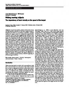
2.3.1 The network In general, a network channels the traffic. This observation holds for road traffic as well as for railway traffic. Air traffic also follows a (three-dimensional) network of air corridors and shipping is strongly influenced by rivers, channels, and other waterways. Even the motion of pedestrians follows a network. Herds of animals often follow a (invisible) network during their migration. In consequence, (almost) no objects can be observed outside of the network. Figure 1 shows two examples. Statement 1: Moving real-world objects very often follow a network.

Figure 1:

Usage of motorways in Northwest Germany (left) and migration of butterflies (right).

In the most cases, a moving object tries to use the fastest path to its destination. Therefore, it does not use an arbitrary path through the network but a path, which is the fastest or not far away from the fastest path. This observation corresponds to the statement in [14] concerning the non-chaotic motion of real-world objects. In some cases, not the speed but other optimization goals (security, beautifulness etc.) may determine the path of the object [13]. Statement 2: Most moving objects use a fast path to their destination.

6

A further observation concerns the connections within the network. Typically, we find connections of different types. In a road network, for example, we find different road classes like motorways, federal roads, secondary roads, minor roads, side roads and so on. This observation also holds for other means of transport. The class may also consider other aspects of a road like the topography, urban areas, and speed limits [13]. The class of a connection has direct impact on the motion of objects: Especially, the speed of the objects is influenced by the class of the connection: high-class connections as motorways generally allow a higher speed than low-class connections, see also table 1. Statement 3: Networks consist of classified connections, which have impact on the speed of spatiotemporal objects. cars 50 90 110 130

in cities outside of cities expressways motorways

Table 1:

campers 50 80 80 100

trailers 50 70 70 80

motor bikes 50 90 110 130

Speed limits (in kph) in Italy according to road classes and types of vehicles.

2.3.2 The traffic The speed of moving objects is not only influenced by the class of the connections but also by other moving objects. Traffic jams are a common experience of road users: If the number of vehicles using a street exceeds a threshold, the maximum and the average speed of the objects will decrease [25]. The threshold depends on the capacity of the connection, which is in general dependent on the class of the connection [3]. Statement 4: The number of moving objects will influence the speed of the objects if a threshold is exceeded. The traffic influences not only the speed of the objects but also their paths. According to statement 2, a moving object tries to use the fastest path to its destination. If a traffic jam occurs, the driver may use a detour because of his or her experience or because of a message of the radio traffic service or of other information providers. Another example is the air traffic where flight controllers divert aircrafts to other air corridors. Statement 5: The path of moving objects may change if the speed on a connection is modified.

7

2.3.3 External impacts There exist further impacts on the number and on the speed of moving objects. The most prominent examples are time and weather conditions. For example, rush hours depend on the time of day and of the weekday. During night, the average speed of vehicles is reduced [13]. Holiday periods are another example where the number of cars and aircrafts increases [26]. Furthermore, special weather conditions (rain, snowfall) may decrease the maximum speed of the moving objects. Statement 6: The number of moving objects is a time-dependent function. Statement 7: The speed of moving objects is influenced by a spatiotemporal function, which is independent of the network and of the objects moving on the network.

2.3.4 The moving object The maximum speed of moving objects differs. Especially, it depends on the class of the moving object. For example, private cars generally have a higher maximum speed than trucks (see table 1). The maximum speed of trucks depends on their weight category [3]. For other means of transport or different animals, this observation holds. Note that other restrictions (statements 3, 4, 6, and 7) may cause that an object will never reach its maximum speed limit. Statement 8: Moving objects belong to a class. This class restricts the maximum speed of the object.

2.3.5 Time-scheduled traffic The motion in public transport systems but also – on special parts of the network (e.g. ferry lines) – of individual vehicles is controlled by time schedules. These time schedules influence the moving objects in respect to their speed (e.g. waiting periods occur) and the path they use (e.g. many car drivers will avoid a ferry if the waiting period is too long). Furthermore, the transition of timescheduled traffic into individually moving objects (e.g. when cars leave a ferry or a railway ferry) may cause congestions. Figure 2 illustrates this effect. The coordinated take-offs and landings of aircrafts on an airport can also be considered as (a special case of) time-scheduled traffic. Statement 9: Time-scheduled traffic may influence the speed and the paths of moving objects.

8

scheduled connection

concentration

concentration

time 1

Figure 2:

time 2

time 3

congestion

time 4

Illustration of the impacts on scheduled connections

2.3.6 Discussion In this section, nine statements are presented concerning the behavior of moving objects. These statements surely do not consider all possible aspects of the movement of objects, but the use of a network requires observing them. Many of the nine statements are motivated by the requirements of applications from the field of traffic telematics based on the experience of the author. The examples presented show that most of them do not only hold for vehicles but for a wide range of moving objects. Many of the above statements are difficult to fulfill without using a network. Especially the concentration of moving objects on few (not necessarily rectilinear) line connections cannot be reached without a network. Because such concentrations are typical for many types of traffic, a benchmark for spatiotemporal database systems should consist of data distributions, which include such hotspots. Furthermore, the generators presented in section 2.2 cannot obtain a speed control, which considers the maximum speed on classified connections and their maximum capacity.

3. The Network-Based Generation of Spatiotemporal Data According to statement 1, moving objects tend to follow a predefined network. Therefore, the basic data structure for generating spatiotemporal objects is a network. In principle, it is possible to generate a synthetic network or use real data. There exist several reasons for using a real network. First, it is not a simple task to generate a network, which has the properties of a real-world network. Second, the use of a network from a real-world application supports the generation of objects, which behave like the objects in this application. Finally, several providers offer real-world networks: The SEQUOIA 2000 Storage Benchmark [20] comprises two (directed) graphs

9

representing drainage networks. Another popular source for test data are the TIGER/Line files of the US Bureau of the Census [23]. These data files comprise detailed road and railway networks.

3.1 The Modeling of Time For generating spatiotemporal objects, a model of time is required. First, we assume that a period T restricts the existence of spatiotemporal objects, i.e. for each object obj.timei ∈ T. T is bounded by a minimum time tmin and a maximum time tmax. In real life, time is continuous. However, for the generation of spatiotemporal objects we have to assume that T is divided by nt+1 time stamps ti into nt time intervals [ti, ti+1) with t0 = tmin, tnt = tmax and ti+1 - ti = ∆t = (tmax - tmin) / nt. All these parameters are globally defined.

3.2 Requirements on the Network The statements of section 2.3 describe some requirements on the connections, i.e. on the edges of the network: •

Each edge belongs to one edge class edgeClass(edge) and for each edge class a maximum speed edgeClassMaxSpeed(edgeClass) is defined (statement 3).

•

The current maximum speed on an edge edgeMaxSpeed(edge) has an individual value equal or less than the maximum speed according to the edge class: edgeMaxSpeed(edge,time) ≤ edgeClassMaxSpeed(edgeClass(edge))

•

Furthermore, for each edge class a maximum capacity edgeClassCapacity(edgeClass) is defined. If the number of objects traversing an edge during a time interval edgeUsage(edge,time) is greater than the maximum capacity of the edge class, the maximum speed on the edge is restricted by a further limit described by a function deceleratedSpeed (statement 4): edgeMaxSpeed(edge,time) ≤ deceleratedSpeed(edgeClass(edge),edgeUsage(edge,time)) , if edgeUsage(edge,time)) > edgeClassCapacity(edgeClass(edge))

Apart from the definition of the class-specific functions (edgeClassMaxSpeed, edgeClassCapacity), these requirements need the following attributes for each edge of the network:

10

•

The attribute edgeClass defines the class of the edge. This attribute is constant; it does not change over the time. A real-world network used for the data generation should define this attribute.

•

The attribute edgeUsage corresponds to the number of objects traversing the edge during a time interval. Its default value is 0; it changes over the time.

Furthermore, we assume that each edge has a time-independent spatial location loc.

3.3 Requirements on the Moving Objects The statements of section 2.3 have also impacts on the modeling of the moving objects: •

Each moving object belongs to an object class objClass(obj) and for each object class a maximum speed objClassMaxSpeed(objClass) is defined (statement 8).

•

The speed of an object on an edge objSpeed(obj,edge,time) is restricted by the maximum speed of its object class and the maximum speed on the edge: objSpeed(obj,edge,time) ≤ objClassMaxSpeed(objClass(obj)) objSpeed(obj,edge,time) ≤ edgeMaxSpeed(edge,time)

Again, a function has to be defined (objClassMaxSpeed) and each object requires an (nonchanging) attribute objClass defining its class.

3.4 External Objects In order to simulate weather conditions or similar events with impact on the motion and speed (statement 7), we introduce extended spatial objects. We can distinguish different types of such external objects: •

External objects, which exist over the whole time, and external objects, which are created at time1 and deleted at time2 (time1 < time2).

•

Static and moving external objects.

11

•

External objects having a static shape and external objects, which change their spatial extension over the time.

The basic properties of such external objects are: •

The position and extension of the object area(extObj,time). The attribute area may change over the time. In the following, it is assumed that a rectilinear box describes the area of an external object. Figure 3 depicts such rectangles computed by the generator.

•

The affiliation to an object class objClass(extObj), which describes basic properties like the speed and the lifetime of an external object. The speed reduction in the area of an external object is determined by the attribute decreasingFactor of the corresponding object class.

Now, a further limit to the maximum speed on an edge can be defined: edgeMaxSpeed(time,edge) ≤ edgeClassMaxSpeed(edgeClass(edge)) ⋅ minimum ({decreasingFactor(objClass(extObj)) with loc(edge) ∩ area(extObj,time) ≠ Ø})

Figure 3:

External objects represented by rectangles.

3.5 Computing the Motion

3.5.1 The lifetime of a moving object According to statement 6, the number of moving objects is a time-dependent function. In order to fulfill this requirement, the creation of new moving objects is controlled by a function

12

numberOfNewObjects(time), which computes the number of new objects at one time stamp. A moving object “dies” when it arrives at its destination or after the maximum time stamp is reached.

3.5.2 The starting node of a moving object Before an object can move, it is necessary to determine its start position. It is assumed that this start position is a node of the network, the so-called starting node. In the following, three different approaches for computing starting nodes are presented and discussed. 1. The data-space oriented approach (DSO) The idea is to compute a position (x,y) by using a two-dimensional distribution function like in [22] and to determine the nearest node of the network. This node is the starting node of the moving object (see figure 4). Assuming a uniform distribution, the result of this approach is that at nodes, where the network is sparse, more objects start than at nodes, where the network is dense. In the example of figure 4, we find concentrations of starting nodes on roads bordering empty areas of the map. These concentrations are indicated by ovals. This behavior contradicts the experience and expectation that in areas where the network is sparse also the demand for entering the network is low.

(x,y)

computing a position (x,y)

using the nearest node as starting point

Figure 4:

Illustration and example of the data-space oriented approach.

2. The region-based approach (RB) In order to improve the behavior of the data-space oriented approach it is necessary to adapt the data distribution to the network. This can be achieved by introducing a tessellation of the data space. Each cell (or more general each region) consists of a value describing the probability of the cell as place of starting nodes. In a real-world application,

13

e.g., the population density of an area may be a suitable measure for this probability. Again, after computing a position (x,y) the nearest node of the network is determined. In the left example of figure 5, the probability of having a starting point in the region of the city center – indicated by the circle – has been 9 times higher than in the outer region. This approach allows an interesting extension: Using the destination node of the route, the probability of a region containing this node can be increased, and using the starting node, the probability of the corresponding region can be decreased. This extension allows (together with a suitable definition of the function numberOfNewObjects) simulating effects like the movement of office workers to downtown in the morning and their return in the evening. 3. The network-based approach (NB) The idea of the last approach is to select a node by using a one-dimensional distribution function. Assuming a uniform distribution, each node is selected with the same probability. In this case, the distribution of the starting nodes is correlated to the density of the network; this effect is illustrated by the right example in figure 5.

Figure 5:

Example for the region-based approach (left) and the network-based approach (right).

The starting node of a moving object is computed by the function computeStartingNode(time).

3.5.3 The destination of a moving object An obvious idea for computing the destination of a moving object is to use the same approach as for determining the starting node. However, this leads to non-satisfying results:

14

The most important objection concerns the length of the routes. Computing the destination independently of the starting node leads to an uncontrolled distribution of the lengths of the paths. However, in real applications this distribution is not arbitrary but correlates to distinct regularities. In cities for example, short drives predominate. The (average) length of routes often correlates to the type of the moving object; e.g., trucks often have longer drives than small private cars [3]. Another influencing factor may be the starting time. Therefore, the preferred lengths of routes are determined by a user-defined function computeLengthOfRoute(time,objClass). Often different distributions for computing the starting nodes and the destination nodes are required. For the example of office workers, it is reasonable to assume that the distribution of starting nodes corresponds to the population density. However, the distribution of the destinations nodes surely does not correspond to this measure. For them, the density of places of work is a much better distribution. Therefore, destination nodes are determined by a separate function computeDestinationNode(time,startingNode,length) getting the starting node and preferred length of the route as additional parameters.

3.5.4 The movement of the objects Each object obj moves between two time stamps ti and ti+1 from its current position obj.loci to its new position obj.loci+1 according to its computed route. In general, these positions do not match with the nodes of the network. The generator logs these positions. For the edges traversed between the two time stamps ti-1 and ti, the number of traversing objects (edgeUsage) is decremented, and for the currently traversed edges, this number is increased.

3.5.5 Computing the route According to statement 2, the route computation should try to find a fast path to the destination following the connections of the given network. This can be achieved by using a traditional routing algorithm. It is not necessary to compute the fastest path but a route that is not much slower than the fastest path. In section 3.3, the requirements on the object speed (objSpeed) have been described. The routing algorithm must consider these requirements by weighting the edges correspondingly.

15

Computing the route at the generation time of an object assumes that the speed of the object on an edge will not change after the computation. However, this assumption contradicts the statements 4 and 5. One solution for this contradiction is to compute a new route at each time stamp. However, such an approach would require a huge computing power. Therefore, it cannot be considered as an adequate solution. Furthermore, that approach is not realistic for a real-world application. In general, we can distinguish two situations where a new “computation” of a route is triggered: First, by an external event (e.g. a message of the radio traffic service) or, second, by a strong deviation of the current speed from the expected speed (e.g. if the car is in a traffic jam). In both cases, the moving object (or its driver) may compute a different route if enough time has passed since the last computation. In order to simulate this behavior, two user-defined boolean functions are introduced: 1. computeNewRouteByEvent (time, timeOfLastComputation) This function allows simulating external events. In a simple version, it may return “true” if time minus timeOfLastComputation is larger than a given threshold. 2. computeNewRouteByComparison (time, timeOfLastComputation, currentSpeed, expectedSpeed) This function allows simulating the reaction in the case of a strong deviation between the current speed and the expected speed on an edge.

3.6 Requirements of Experiments In this section, requirements are discussed, which do not have the goal to simulate realistic moving objects, but to meet the requirements of typical experiments. These requirements are based on the feedback of the first groups using the generator.

3.6.1 Constant number of objects Experiments often need a constant number of investigated objects during the whole period T, e.g., for estimating the cost of an algorithm. However, the approach presented in section 3.5 cannot guarantee an exact number of objects, but only an approximate number of objects after an initial phase if the return value of the function numberOfNewObjects(time) is constant. In order to support a constant number of objects, a method reachDestination (destinationNode) is called when an object reaches its destination. This method can be used, for example, for influencing the behavior

16

of the function numberOfNewObjects (e.g. returning how often reachDestination has been called since the last invocation of numberOfNewObject) and of the function computeStartingNode (e.g. returning a destinationNode obtained by reachDestination as the new starting node).

3.6.2 Report probability There are often situations where a moving object reports its position irregularly. Examples are applications where the objects will transmit their location only if a special event occurs. For an observer, the position of such an object does not change at every time stamp but only when a new location is transmitted. For supporting such situations, a function getReportProbability (objClass) exists defining for each object class a probability that a move is reported during a time interval.

4. The Framework The generation of network-based spatiotemporal data requires the following steps: 1. the preparation of the network, 2. the definition of the required (user-defined) parameters and functions, 3. the computation of the moving objects and of the external objects, and 4. the report of the computed objects. We have built up a framework for performing these four steps. This framework is based on the programming language Java that allows using the generator on all important computer platforms and operating systems.

4.1 The Preparation of the Network The generator can read the network representation either from files or from an Oracle database. In the first case, two binary files describe the nodes and the edges of the network according to a simple syntax. In order to use existing network files and benchmark data, tools can be used to transform them into this file format. Currently, two tools exist which allow using TIGER/Line Files [23] and MapInfo Data Interchange Format (MIF) Files [9]. Figure 6 shows examples of such road networks. Besides, the option exists that the network is stored in an Oracle database using the

17

object-relational geometry type of Oracle Spatial [11]. In this case, the generator transforms sets of lines stored without an explicit topology automatically into a network.

Figure 6:

Example networks: City of Stockton in San Joaquin County, CA. (left) City of Oldenburg, Germany (right)

4.2 The Definition of Parameters and Functions The simplest techniques to control a program are interactive parameters and the use of parameter files. Both techniques are supported by the generator. Figure 7 shows the input panel allowing the input of basic parameters and a part of a typical parameter file allowing the definition of more sophisticated parameters.

! limits of input fields MIN_MAXTIME = 5 MAX_MAXTIME = 400 MAX_OBJCLASSES = 20 ! settings of the generator urlnez = file:/E:/Java/Data DSO VIZ outputFile = oldenburg.txt ! settings of the applet viewWidth = 500 viewHeight = 500 language = E color = white

Figure 7:

Controlling the generator by an input panel and a parameter file.

However, section 3 has demonstrated that a network-based generation of spatiotemporal data requires a large variety of user-defined functions and parameters. Their behavior and complexity

18

depend on the real-world application, which should be simulated. Therefore, it is difficult to establish an environment where all these functions and parameters can be defined by a simple user interaction or by predefined parameter files. For that reason, the generator allows and supports the users to program these functions and parameters themselves in Java. This a simple task because the corresponding class files are already predefined; only their functionality must be adapted. The dynamic class-loading feature of Java simplifies the integration of these user-defined classes into the generator. As a result, it is no problem to integrate newly compiled classes as long as their interface does not differ from the previous versions of the object classes. Appendix B lists the object classes and operators, which can be defined by the user. The input parameters of the algorithm in appendix A correspond to the basic input parameters of the generator.

4.3 The Computation The most important aspects of the computation have been described in section 3. The algorithm describing the sequence of computations is presented in appendix A. The routing algorithm used by the generator is a modification of Dijkstra’s algorithm, the A* algorithm [1]. The data-space oriented approach and the region-based approach for determining a starting or destination node require nearest-node queries. External objects determine covered edges of the network by performing window queries. Therefore, the generator uses a main-memory based r-tree [6] having a small node capacity.

4.4 The Report The generator supports three types of reporting: •

the report into a simple text file,

•

the report into a JDBC database, and

•

an ad-hoc visualization of the generated objects (see figure 8).

The generator allows reporting the positions of the moving objects during their lifetime, the nodes of the network passed by the moving objects during their lifetime, and the positions and extensions of the external objects during their lifetime. The user can overwrite all reporting functions. Hence,

19

any user-defined data format can be supported. The generator can be run as Java application and as Java applet. Using the second option, it is possible to run the generator via the Internet. Changing a scrollbar that represents the time axis allows visualizing the motion of the objects (see figure 9).

Figure 8: Visualization of moving objects of all time stamps (color = object class) (left: City of Stockton in San Joaquin County; right: City of Oldenburg)

Figure 9:

Visualization of moving objects during consecutive time stamps (whole San Joaquin County)

4.5 Promoting the Generator by a Web Site In order to make benchmark data tools available for other users, typically a web site is being prepared which allows downloading the tool (e.g. the generator), the user documentation, and data files (see also [21]). For the generator presented in this paper, the reader will find such a web site under http://www.fh-wilhelmshaven.de/oow/institute/iapg/personen/ brinkhoff/generator.shtml. In addition, source files of classes with user-defined functions

are provided as examples.

20

As mentioned before, the generator can be run as a Java applet. This allows providing a demonstration applet of the generator without any further actions like downloading and installation. The visitor of the page immediately gets an impression whether this tool may be suitable for her or his application. The visitor can immediately visualize the generated objects and their motion.

5 Performance Issues The network-based generation of spatiotemporal datasets is – of course – much costlier than a generation where the objects are distributed over the data space according to a given or userdefined distribution function. A question arises: •

Is the presented approach (based on Java as programming language) able to produce datasets in a reasonable time?

The run time of the generator depends on many influencing factors. Therefore, we can give here only an impression of the performance of the generator. The following performance measurements have been done on a standard personal computer with an Intel Pentium III 500 MHz processor, 128 MB main memory and Microsoft Windows NT as operating system. The Java 1.1 code has been performed by the Microsoft Virtual Machine for Java 5.0 with an activated just-in-time compiler. Several test series with different datasets and parameter settings have been performed. The first presented group of test series is based on the road network of the City of Oldenburg, which contains of 5,835 nodes and 6,065 edges. The average degree of the nodes in this network is 2.63. The number of object classes has been 6. The network-based approach for determining a starting node has been used and no external objects have been generated. The probability for the computation of a new route by an event has been 0.5% per move of an object and the probability for the computation of a new route has been 5% per edge if the capacity of the edge was exceeded. The maximum speed of the fastest object class on the fastest connection has been 4% of the extension of the data space in one dimension. The object classes, which can be downloaded as examples from the web site mentioned in section 4.5, give the exact definition of the behavior of the generator for the tests. Furthermore, the complete test protocols can be downloaded there. Table 2 depicts the major results of the experiments.

21

# route total time total time / total time / test # time # objects / # objects # points computations (sec) object (msec) node (msec) number stamps time stamp O-1-1 100 10 1,000 33,582 1,139 23 23.4 0.48 O-1-2 200 10 2,000 86,353 2,421 48 24.0 0.51 O-1-3 400 10 4,000 200,424 5,109 106 26.3 0.52 O-1-4 800 10 8,000 496,908 10,741 217 27.1 0.52 O-1-5 1,600 10 16,000 1,051,861 21,877 467 27.2 0.55 O-2-1 100 20 2,000 68,811 2,448 43 21.4 0.44 O-2-2 200 20 4,000 189,702 5,251 105 26.3 0.50 O-2-3 400 20 8,000 491,563 11,230 224 28.0 0.51 O-2-4 800 20 16,000 1,190,768 23,854 532 33.2 0.57 O-2-5 1,600 20 32,000 2,570,035 48,823 1,063 33.2 0.56 O-3-1 100 40 4,000 149,605 5,114 94 23.5 0.45 O-3-2 200 40 8,000 445,118 11,291 202 25.2 0.45 O-3-3 400 40 16,000 1,222,477 25,173 504 31.5 0.52 O-3-4 800 40 32,000 2,973,494 53,599 1,057 33.0 0.52 O-3-5 1,600 40 64,000 6,702,669 111,552 2,272 35.5 0.54 O-4-1 100 80 8000 331,102 10,701 191 23.9 0.44 O-4-2 200 80 16,000 1,061,260 24,129 438 27.4 0.47 O-4-3 400 80 32,000 3,000,485 53,590 1,011 31.6 0.51 O-4-4 800 80 64,000 7,425,420 114,631 2,208 34.5 0.54 O-4-5 1,600 80 128,000 16,514,148 237,215 4,535 35.4 0.55

Table 2:

Results of the Oldenburg test series.

The second group of test series is based on the road network of San Joaquin County (source: TIGER/Line Files). This network consists of 18,496 nodes and 24,123 edges with an average node degree of 3.14. The other test conditions have been the same as in the first experiments. Table 3 depicts the main results of these test series. # route total time total time / total time / Test # time # objects / # objects # points computations (sec) object (msec) node (msec) number stamps time stamp S-1-1 100 10 1,000 28,685 1,158 183 182.5 1.86 S-1-2 200 10 2,000 73,133 2,465 406 203.0 1.92 S-1-3 400 10 4,000 174,233 5,081 845 211.3 1.99 S-1-4 800 10 8,000 388,366 10,455 1,765 220.7 2.03 S-1-5 1,600 10 16,000 866,142 21,537 3,848 240.5 2.16 S-2-1 100 20 2,000 62,145 2,511 404 202.0 1.91 S-2-2 200 20 4,000 160,513 5,398 845 211.1 1.92 S-2-3 400 20 8,000 384,526 11,148 1,781 222.7 2.00 S-2-4 800 20 16,000 886,037 23,110 3,657 228.5 1.99 S-2-5 1,600 20 32,000 1,964,940 47,877 7,990 249.7 2.08 S-3-1 100 40 4,000 133,887 5,435 791 197.8 1.77 S-3-2 200 40 8,000 372,666 11,712 1,641 205.2 1.77 S-3-3 400 40 16,000 933,470 25,228 3,668 229.2 1.87 S-3-4 800 40 32,000 2,192,473 52,523 7,837 244.9 1.92 S-3-5 1,600 40 64,000 4,904,090 108,914 16,761 261.9 1.98 S-4-1 100 80 8000 292,630 11,210 1,502 187.7 1.66 S-4-2 200 80 16,000 861,086 24,303 3,293 205.8 1.71 S-4-3 400 80 32,000 2,229,659 51,832 6,964 217.6 1.73 S-4-4 800 80 64,000 5,240,853 107,932 15,241 238.1 1.81 S-4-5 1,600 80 128,000 11,642,957 222,103 31,926 249.4 1.84

Table 3:

Results of the San Joaquin County test series.

Following observations can be made: •

It is possible to produce datasets with network-based moving objects on a standard personal computer in a reasonable time: the time per computed point is between 0.3 and

22

0.7 msec for the Oldenburg test series and between 2.7 and 6.5 msec for the San Joaquin County test series. These values allow generating large datasets. •

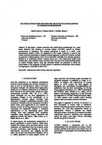
If the density of traffic increases (i.e. the number of new objects computed per time stamp), the number of computed routes initiated by a comparison of the current and the expected speed on an edge will increase. The number of computations initiated by events is also influenced: Because of the increased traffic, the average speed of the objects decreases; in consequence, the number of events per route increases. Figure 10 depicts the number of route computations per object for the test series O-x-3.

1,2

# routes

1 0,8

# initial routes / object

0,6

# routes by event / object

0,4

# routes by comparison / object

0,2 0 O-1-3

O-2-3

O-3-3

O-4-3

Figure 10: The number of computed routes per object dependent on the traffic density. •

The number of routes initiated by events or by comparisons also grows with the number of time stamps because the average lifespan of the objects increases then. Figure 11 illustrates this effect for the test series S-3-x:

1,2

# routes

1 0,8 # initial routes / object

0,6

# routes by event / object

0,4

# routes by comparison / object

0,2 0 S-3-1

S-3-2

S-3-3

S-3-4

S-3-5

Figure 11: The number of computed routes per object dependent on the lifetime. •

In order to neglect the effects caused by the increased number of computed routes, the last column in table 2 and table 3 shows the computing time per node traversed by the routes. We can observe that this value is relatively constant for each of the test series.

23

•

The computing time per object especially depends on the chosen network; this time is about 10 times higher for the second test series than for the first. The first reason for this observation is the higher number of traversed nodes per route for the San Joaquin County test series (factor about 2.1). However, this factor does not explain the whole difference. The other important reason are the different average node degrees: 2.63 compared to 3.14. For computing a route in the Oldenburg network, there exist 0.63 wrong paths on the average per node, which must be considered by the routing algorithm, whereas in the San Joaquin County network this number is 1.14.

The use of external objects decreases the speed of the generator by a factor of about 2. Comparative measures using the Symantec Java JustInTime Compiler Version 3.10 for JDK 1.1.x have shown similar results. The generation of native code has not brought any performance gains.

6. Conclusions and Future Work In order to evaluate spatiotemporal database systems or their components (e.g. access methods), it is necessary to define benchmarks. Such a benchmark demands datasets simulating the typical behavior of moving objects. First approaches to generate such datasets have been published recently ([22], [14], [12]). However, one important property of moving objects has not been considered so far: In many applications dealing with spatiotemporal data (e.g. in the field of traffic telematics), the objects follow a given network. Therefore, benchmarks require datasets with such “network-based” moving objects. This paper deals with the generation of network-based moving objects. In order to specify the behavior of such objects, nine statements have been presented and discussed. These statements have been the starting point for the specification and development of a new generator for spatiotemporal data. This tool generates synthetic data based on real data. Important issues of the generator are: •

The computation of the objects is based on a network.

•

Edge classes limit the maximum speed on edges and their maximum capacity. The class of a moving object also limits its speed.

•

Moving external objects decrease the speed of the moving objects in their varying vicinity. 24

•

Different approaches for determining the starting point and the destination node of a moving object are supported. The length of the route between these two nodes can be controlled.

•

A dynamic re-computation of a route may be initiated by a reduced speed on an edge or by an external event.

A framework for preparing the network, for defining parameters and user-defined functions, for generating the moving objects, and for reporting the computed objects have been presented. The investigation of the performance of the generator shows that it is possible to produce datasets of network-based moving objects on a standard PC in reasonable time. In order to promote the generator, a web site has been prepared which allows downloading the generator, its documentation and examples of classes with user-defined functions. In addition, an interactive applet demonstrating the generator can be found there. Two concepts generalizing the generation process have not been integrated into the current implementation of generator yet: the support of moving objects, which follow the network only approximately, and the support of three-dimensional moving objects: In the presented approach, the moving objects follow the network strictly. However, in many applications the moving objects follow the network only approximately. Examples are air traffic and sea traffic. In those cases, we have to allow a deviation of the object from the edges of the network. A simple solution is to shift the position of the object by a random direction and (restricted) random distance. However, this approach often leads to a zigzag course. Figure 12 gives an example. Such a movement is mostly not very realistic (an exception are delivery patterns of mail(wo)men or similar delivery activities).

strict movement

zigzag movement

Figure 12: Zigzag movement

25

In order to avoid such a zigzag movement, it is more reasonable not to compute a new deviation at each time stamp but to change the deviation a little bit at each time stamp. This leads to a more regular (and realistic) movement like in figure 13. regular movement

strict movement

Figure 13: Regular movement For simulating air traffic, the third dimension has to be considered. One solution is to build up a three-dimensional network and to use it as described in section 3. Another approach is to derive the information about the height “on the fly”, i.e. to define a function computeHeight which computes the z-coordinate. The movement of an aircraft can be divided into the take-off phase, the flight on a given height and the landing. The function computeHeight simulates the behavior of the aircraft during these three phases; it needs the distance of the current position of the object to the starting and the destination node to select the right phase and the complete distance and the class of the object to compute the flying height.

9. References [1]

R.K. Ahuja, T.L. Magnanti, and J.B. Orlin. Network Flows: Theory, Algorithms, and Applications, Prentice-Hall, 1993.

[2]

T. Brinkhoff. Requirements of Traffic Telematics to Spatial Databases, in Proceedings 6th International Symposium on Large Spatial Databases, Hong Kong, China. Lecture Notes in Computer Science, Vol.1651:365-369, 1999.

[3]

Bundesanstalt für Straßenwesen, Bundesrepublik Deutschland. http://www.bast.de/

[4]

J. Gray. The Benchmark Handbook, Morgan-Kaufman, 1991.

[5]

O. Günther, V. Oria, P. Picouet, and J.-M. Saglio, M. Scholl. Benchmarking Spatial Joins Á La Carte, in Proceedings 10th International Conference on Scientific and Statistical Database Management, Capri, Italy, pp. 32-41, 1998.

[6]

A. Guttman. R-trees: A Dynamic Index Structure for Spatial Searching, in Proceedings ACM SIGMOD International Conference on Management of Data, Boston, MA, pp. 47-57, 1984.

[7]

Integrating Spatial and Temporal Databases, Seminar, Schloss Dagstuhl, Wadern, Germany, November 22–27, 1998.

[8]

H.-P. Kriegel, M. Schiwietz, R. Schneider, and B. Seeger. Performance Comparison of Point and Spatial Access Methods, in Proceedings 1st Symposium on the Design and Implementation of Large Spatial Databases, Santa Barbara, CA. Lecture Notes in Computer Science, Vol. 409: 89-114, 1989.

26

[9]

MapInfo Corporation. MapInfo ProfessionalTM: Reference Manual, 1995.

[10]

H. Mehl. Mobilfunk-Technologien in der Verkehrstelematik, Informatik-Spektrum, Vol. 19:183-190, 1996.

[11]

Oracle Corporation. Oracle® Spatial, User’s Guide and Reference, Release 8.1.7, 2000.

[12]

D. Pfoser and Y. Theodoridis. Generating Semantics-Based Trajectories of Moving Objects, in Proceedings International Workshop on Emerging Technologies for Geo-Based Applications, Ascona, Switzerland, pp. 59-76, 2000.

[13]

RandMcNally. The Road Atlas: United States, Canada & Mexico, 2001.

[14]

J.-M. Saglio and J. Moreira. Oporto: A Realistic Scenario Generator for Moving Objects, in Proceedings DEXA Workshop on Spatio-Temporal Data Models and Languages, Florence, Italy, pp. 426-432, 1999. An extended version is published in: GeoInformatica 5(1):71-93, 2001.

[15]

T. Sellis. Research Issues in Spatio-temporal Database Systems, in Proceedings 6th International Symposium on Large Spatial Databases, Hong Kong, China, Lecture Notes in Computer Science, Vol. 1651:5-11, 1999.

[16]

B. Seeger, M. Egenhofer, J. Gray, S. Leutenegger, and D. Papadias. Seeking the Truth – Curses and Blessings of Experiments, Panel of the 7th International Symposium on Spatial and Temporal Databases, 2001.

[17]

Spatial and Temporal Databases, 7th International Symposium, Redondo Beach, CA, July 1215, 2001.

[18]

Spatio-Temporal Database Management, Workshop, Edinburgh, Scotland, September 10-11, 1999.

[19]

Spatio-Temporal Data Models and Languages, Workshop, Florence, Italy, August 30-31, 1999.

[20]

M. Stonebraker, J. Frew, K. Gardels, and J. Meredith. The SEQUOIA 2000 Storage Benchmark, in Proceedings ACM SIGMOD International Conference on Management of Data, Washington, DC, pp. 2-11, 1993.

[21]

Y. Theodoridos and M. Nascimento. Generating Spatiotemporal Datasets on the WWW. ACM SIGMOD Record, Vol. 29(3):39-43, 2000.

[22]

Y. Theodoridis, J.R.O. Silva, and M.A. Nascimento. On the Generation of Spatiotemporal Datasets, in Proceedings 6th International Symposium on Large Spatial Databases, Hong Kong, China, Lecture Notes in Computer Science, Vol. 1651:147-164, 1999.

[23]

U.S. Government Information and Maps Department. The Map Collection - TIGER/Line Files, http://www.lib.ucdavis.edu/govdoc/MapCollection/tiger.html

[24]

J. Zobel, A. Moffat, and K. Ramamohanarao. Guidelines for Presentation and Comparison of Indexing Techniques. ACM SIGMOD Record, Vol. 25( 3):10-15, 1996.

[25]

3sat: Raus aus dem Stau, Ein nano-Schwerpunkt. http://www.3sat.de/nano/bstuecke/18130/index.html

Appendix A The following code describes the sequence of computations done by the generator. The principal input parameters are listed as parameters of the operation computeMovingObjects.

27

operation computeMovingObjects ( Network network, // the network int maxTime, // the maximum time stamp int numOfObjClasses, // the number of classes of moving objects int numOfObjAtBegin, // number of external objects at the beginning int numOfObjPerTime, // number of new moving objects per time stamp int numOfExtObjClasses, // number of classes of external objects int numOfExtObjAtBegin, // number of external objects at the beginning int numOfExtObjPerTime, // number of new external objects per time stamp int speedDivisor, // controls the general speed of the objects int reportProbability, // indicates the general report probability Properties prop // parameters of the property file ) { // The initialization of the different objects classes using the above parameters and // the parameter file is omitted. They get the parameters listed above. // Then, the time starts. time.init(); while not time.maximumTimeIsExceeded() do { int currTime = time.getCurrentTime(); // move all existing external objects and report their new positions and extensions // if an external object dies, it is removed from the container for all extObj in containerOfExternalObjects do { extObj.moveAndResize (currTime); if extObj.isDead() then { reporter.reportDisappearingExternalObject(currTime,extObj); containerOfExternalObjects.remove(extObj); } else reporter.reportExternalObject(currTime,extObj); } // move all existing objects and report their new positions // if necessary, a new route is computed // if an object has reached its destination, it is removed from the container for all obj in containerOfMovingObjects do { if reRoute.computeNewRouteByEvent(obj,currTime) then obj.reroute(network); obj.move (currTime,network,reroute,reporter); // 'move' performs also a rerouting triggered by "comparison" if obj.hasDestinationReached() then { objectGenerator.reachDestination(obj.getDestinationNode()); reporter.reportDisappearingObject(currTime,obj); containerOfMovingObjects.remove(obj); } else reporter.reportMovingObject(currTime,obj,reportProbability); } // generate, store and report new external objects for i = 1 to externalObjectGenerator.numberOfNewObjects(currTime) do { ExternalObject extObj = externalObjectGenerator.computeExternalObject(currTime); containerOfExternalObjects.add(extObj); reporter.reportNewExternalObject(extObj); } // for each new moving object... for i = 1 to objectGenerator.numberOfNewObjects(currTime) do { // determine its properties int objClass = objectClasses.computeNewObjectClass(currTime); Node start = objectGenerator.computeStartingNode(currTime,objClass); long length = objectGenerator.computeLengthOfRoute(currTime,objClass); Node dest = objectGenerator.computeDestNode(currTime,start,length,objClass); // create, store and report the object MovingObject obj = new MovingObject(objClass,start,dest,currTime); containerOfMovingObjects.add(obj); reporter.reportNewMovingObject(obj); // and compute its (first) route obj.computeRoute(network); } // go to the next time stamp time.increaseCurrTime(); } }

28

Appendix B In the following, the operations of object classes within the framework are presented, which can be re-defined for controlling the behavior of the generator. The constructors, which can also be redefined by the users, are skipped. Class EdgeClasses // Definition of the properties of the edge classes. int deceleratedSpeed (int edgeClass, int edgeUsage); // Computes the decelerated speed of an edge class // depending on the usage and the capacity of the edge. int getCapacity (int edgeClass); // Returns the capacity of an edge class. int getMaxSpeed (int edgeClass); // Returns the maximum speed of an edge class.

Class ObjectClasses // Definition of the properties of the classes of moving objects. int computeNewObjectClass (int currTime); // Computes the object class of a new moving object. int getMaxSpeed (int objClass); // Returns the maximum speed of an object class. int getReportProbability (int objClass) { // Returns the report probability of an object class.

Class ExternalObjectClasses // Definition of the properties of the classes of external objects. int computeNewExternalObjectClass (int currTime); // Computes the object class of a new external object. int getDecreasingFactor (int objClass); // Returns the factor of the class for the decreasing the speed in per cent. // Additional user-defined functions for describing the size, the lifetime, and the change // of external objects used by the user-defined class “ExternalObjectGenerator” belong to // this class.

Class ObjectGenerator // Generator for new starting and destination nodes of moving objects. int numberOfNewObjects (int currTime); // Returns the number of new objects at a time stamp. Node computeStartingNode (int currTime, int objClass); // Computes a new starting node. int computeLengthOfRoute (int currTime, int objClass); // Generates the length of a new route. Node computeDestNode (int currTime, Node startingNode, int length, int objClass); // Computes a new destination node of a route.

29

void reachDestination (Node destinationNode) ; // Is called, when a moving object reaches its destination. // Can be used for influencing the behavior of the methods "numberOfNewObjects", // "computeDestinationNode", and "computeStartingNode".

Class ExternalObjectGenerator // Generator for creating and changing external objects. ExternalObject computeExternalObject (int currTime); // Computes a new external object. Rectangle computeNewPositionAndSize (int currTime, ExternalObject obj) { // Computes the new position and size of an external object. int numberOfNewObjects (int currTime); // Returns the number of new external objects at a time stamp.

Class ReRoute // Class which decides about the re-routing. boolean computeNewRouteByComparison (int lastTime, int currTime, int origSpeed, int actSpeed); // Decides whether a route should be recomputed because of the comparison or not. boolean computeNewRouteByEvent (int lastTime, int currTime); // Decides whether a route should be recomputed or not because of an event.

Class Reporter // Class for reporting the computed moving and external objects. // All operations of this class may be adapted to the requirements of the user.

30

Author Biographics

Thomas Brinkhoff Received his Diploma Degree in Computer Science from the University of Bremen, Germany, in 1990. In 1991, he became research and teaching assistant at the Institute of Computer Science at the University of Munich, where he got his Doctoral Degree in 1994. Between 1995 and 1999, he was project leader for developing GIS applications in the field of traffic telematics at the Mannesmann Autocom GmbH, Düsseldorf. He is currently Professor for Geoinformatics at the Fachhochschule Oldenburg/Ostfriesland/Wilhelmshaven (University of Applied Sciences) in Oldenburg, Germany. His research interests are query and join processing in spatial database systems and the representation and management of moving objects.

31