this paper presents a novel approach for process model test case selection which is able to address flexible user-driven test case selection require- ments and ...
A Genetic Algorithm for Automatic Business Process Test Case Selection Kristof B¨ohmer and Stefanie Rinderle-Ma University of Vienna, Faculty of Computer Science {kristof.boehmer,stefanie.rinderle-ma}@univie.ac.at
Abstract. Process models tend to become more and more complex and, therefore, also more and more test cases are required to assure their correctness and stability during design and maintenance. However, executing hundreds or even thousands of process model test cases leads to excessive test suite execution times and, therefore, high costs. Hence, this paper presents a novel approach for process model test case selection which is able to address flexible user-driven test case selection requirements and which can integrate a diverse set of knowledge sources to select an appropriate minimal set of test cases which can be executed in minimal time. Additionally, techniques are proposed which enable the representation of unique coverage requirements and effects for each process node and process test case in a comprehensive way. For test case selection, a genetic algorithm is proposed. Its effectiveness is shown in comparison with other test case selection approaches. Keywords: Process Modeling and Design, Process Testing, Test Case Selection, Genetic Algorithm
1
Introduction
Over the past years, processes have risen to deeply integrated solutions which are extremely important for various organizations. Hence, ensuring the stability and correctness of processes is a crucial challenge [11]. Several approaches for process verification exist [14], that focus on structural and behavorial correctness of process models. Specifically, when implementing process models, testing has proven a valuable complement to capture the process behavior at runtime, e.g., with respect to process data [18]. Testing concentrates on creating and executing test cases on the tested process model [13]. At minimum a test case consist of input data, which is used to initialize a new instance of the process under test, and an expected execution path that should be followed by the process model instance when executing the test case [18]. A fault can be detected, e.g., when an execution path deviates from the expected test case execution path [18]. Testing plays an important role in process model design, development, and maintenance because it allows to identify faults early during these phases [18]. As process models tend to become more and more complex, manual test case
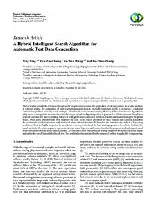
Fig. 1. Test case selection example with coverage illustration
generation becomes time-consuming and, therefore, expensive [17]. Hence, automatic test case generation tools emerged which quickly generate hundreds or even thousands of test cases to completely test a single process model [9]. Each individual test case might be executed quickly. However, executing all test cases may still require an excessive amount of time and, therefore, results in high costs [5]. Hence, it becomes necessary to apply test case selection and minimization techniques. Those techniques select an appropriate1 subset of the available test cases to be executed. If the subset is small and efficient enough then significant time-savings are achieved [5, 12]. Take, for example, the process model shown in Fig. 1. It’s tested by three test cases, whereby the first covers the top most path, the second the middle path and so on. Assume that the user requirement is to cover 75% of the process model (i.e., 75% node coverage, so 75% of all nodes are tested by test cases)2 . Then possible subsets would be to select T1 and T2 (combined execution time 15 minutes), T2 and T3 (25 minutes), or T1 and T3 (20 minutes). However, if the selected test cases should be executed in the minimum possible amount of time then the selection technique must select T1 and T2 as the optimal subset. Identifying an optimal test case subset results in a combinatorial explosion problem [5] (the complexity is exponentially related to the amount of test cases). Hence, it cannot be solved in polynomial time [8]. So, existing approaches utilize heuristics, such as the Greedy Algorithm, which allow to find solutions where analytical algorithms are infeasible because of the huge search space [5]. We have analyzed existing process model test case selection and minimization approaches and found that those are inflexible regarding the supported userdefined coverage requirements, only use a incomprehensive representation of each node’s unique coverage requirements, and also model the coverage effects of each test case in a limited fashion. Hence, existing work is not suitable for answering the following research questions: RQ1 How can node coverage effects for process model test cases be modeled in a more comprehensive way? RQ2 How can the unique coverage requirements of each process node be determined and utilized during process model test case selection? 1
2
Appropriate means that user-defined requirements are fulfilled such as a minimal coverage objective, e.g., that a minimal amount of process nodes is tested. Multiple coverage metrics exist such as path, branch, or node coverage. However, in this paper we will, for the sake of brevity, only use node coverage. However, we are confident that a generalization to other coverage metrics is possible.
RQ3 Is it possible to integrate and utilize more complex process model test case selection requirements than supported by existing work (e.g., to optimize the selected test cases based on their execution time)? RQ4 Whether and how can Genetic Algorithms be utilized to identify an appropriate set of test cases during process model test case selection? In this paper we want to address the identified limitations and concentrate our efforts on test case selection in the process modeling domain. Therefore, we propose a comprehensive representation of test case coverage effects along with a novel approach to identify the unique coverage requirements of each process node. Here we exploit the fact that different kinds of nodes in a process model may have a different complexity, e.g., tasks versus gateways [3]. Additionally, we prove the applicability of Genetic Algorithms for process model test case selection and show, by using an evaluation and a prototypical implementation, that the presented approach supports more complex and flexible selection requirements than existing work. This paper is organized as follows. Coverage metrics, prerequisites, and ways to improve the current situation are discussed in Section 2. Section 3 describes the proposed genetic test case selection approach. Evaluation, corresponding results and their discussion are presented in Section 4. Section 5 discusses related work. Conclusions and future work is given in Section 6.
2
Coverage Metrics
This section introduces coverage metrics for test case selection based on a given process model O. O is defined as directed graph O := (N, CE, DE)3 where N denotes the set of process nodes, CE the set of control flow edges, and DE the set of data flow edges. As auxiliary functions (cf. [15]), we utilize the direct successors of a node n as n• := {n0 ∈ N | (n, n0 ) ∈ CE} for the control flow and n◦ := {n0 ∈ N | (n, n0 ) ∈ DE} for the data flow. The direct predecessors of n can be defined accordingly by •n := {n0 ∈ N | (n0 , n) ∈ CE} for the control flow and ◦n := {n0 ∈ N | (n0 , n) ∈ DE} for the data flow. In this paper, we are mainly interested in the execution path of each test case, especially to determine which process model nodes are covered (i.e., tested) by each test case. So a test case is formally defined as: Definition 1 (Test Case). A test case v on a process model O = (N, CE, DE) is defined as v := (Nv , CEv , enabled) with Nv ⊆ N , CEv ⊆ CE, and enabled ∈ {0, 1} where Nv and CEv form the expected test case execution path and enabled indicates if the test case should be executed (1) or not (0). The ordered set V of all test cases v on a process model O is denoted as test suite, which can be configured to create a test suite configuration Vi where all test cases are enabled or not (i.e., v.enabled is set to 1 or 0). 3
The notion of directed graphs corresponds to the internal representation in order to cover different prevalent process modeling notations such as BPMN [10].
Test case selection starts with a test suite V (consisting of all available test cases for the process model O) and a set of requirements R which are userdefined, such as, the minimal node coverage should be 75%. The requirements contained in R must be satisfied to find a test suite configuration (i.e., deciding which test cases should be executed when executing the test suite) which provides an adequate testing of the process. Hence, the challenge is to find a minimal subset V 0 ⊆ V that satisfies all requirements in R. One typical requirement is that the process must be completely covered (i.e., each node must be tested by the selected test cases). For this, mostly, simple coverage metrics are used. For example, a process node is already marked as completely covered, and therefore, fully tested, when it is checked by at least one test case. However, this approach ignores that each process node has a unique complexity and significance [3] and therefore should be covered by an individually adjusted number of test cases to achieve an optimal coverage. 2.1
Optimal Coverage: Optimal Number of Test Cases per Node
This approach is called optimal coverage because it determines an optimal coverage value (i.e., how many test cases should be used to test it) based on various complexity metrics individually for each process node. We assume that if a process node (e.g., an activity or gateway) is more complex than another one, it must be tested more thoroughly (i.e., covered by more test cases) and, therefore, must be assigned a higher optimal coverage value. We suggest to determine the optimal coverage value Co (j) of node j as the weighted sum over selected complexity metrics compi (j) for node j, (i = 1, . . . , n): & n ' X Co (j) := 1 + wi · compi (j) (1) i=1
In Eq. 1, wi ∈ [0, 1] defines the weight for metric compi (j). Moreover, a minimal coverage of 1 is assigned to each node, i.e., each node must be covered by at least a single test case. The complexity metrics and the weights reflect the process node coverage requirements. One example for a complexity metric is the Fan-In/Fan-Out metric (cf. [7]): for node j it sums over the number of successors |j • | and predecessors | • j| of node j and divides this sum by the maximum Fan-In/Fan-Out value over all nodes of the process model. Two types of metrics are considered in this paper. First, generic metrics that are based on the process model itself which incorporate the node complexity (the structural Fan-In/Fan-Out metric), the process structure (a node is positioned in sequences or more complex loops, error, or concurrent paths), or the node position (a fault at an early executed node affects more follow up process nodes than a fault at a late node). Second, metrics that are supported by historic data (e.g., log files), such as previously identified faults (it is then more likely to find another fault), node execution frequency (an fault does have an higher effect if the faulty node is executed more frequently), previous coverage (if a node was not covered during previous tests, then it should be checked during follow up
tests), error path probability (if a node frequently has to fall back to its error path it more likely contains a fault), frequency of data-modifications (we assume that a node which modifies multiple variables has likely a higher internal complexity than a node which modifies only one variable), and known changes (if a process node is changed then those changes should be checked with tests). Example: Node j has three incoming edges and one outgoing edge. It is analyzed using the Fan-In/Fan-Out metric4 with a weight of 1. Further, the node with the maximum Fan-In/Fan-Out metric of the whole process model has four incoming and two outgoing edges. Then compf an would generate the following result:(1 + 3)/(2 + 4)�= 0.66. The � total optimal coverage can then be calculated by Co (j) using 1 + (1 · 0.66) = 2, i.e., two test cases are required to throughly test j, when considering its complexity. Existing approaches would ignore the node complexity and hence test it with a single test case. This could result in not detecting faults that will be found by the proposed approach. Why? Because, each node has a specific internal node behavior 5 which can, for example, contain multiple execution branches. Imagine that the internal node behavior contains a single conditional branch which provides two execution paths (e.g., for premium or normal customers), then a single test case will most likely only test one of the branches so 50% percent of the node’s internal behavior and it will require at least two test-cases to throughly test the node. Note, that we are assuming that the mentioned complexity metrics also allow to assess the nodes internal complexity (e.g., a node with many incoming edges most likely has a more complex internal behavior then a node with only one incoming edge).
2.2
Test Coverage Metrics: Coverage of all Enabled Test Cases
The following coverage calculation approaches are applied individually on each process node j to determine, given a test suite configuration Vi and a process model O, which test coverage is achieved by Vi on j. Traditional Coverage The traditional coverage is based on existing coverage calculation approaches. The traditional coverage covtr is calculated for a process node j and a test suite configuration Vi by analyzing the test paths of each enabled test case v = (Nv , CEv , 1) (cf. Eq. 2). covtr (j, Vi ) :=
X
counttr (v, j)
(2)
v=(Nv ,CEv ,1) ∈ Vi
If j is covered by an enabled test case (i.e., it is contained in j ∈ Nv of v = (Nv , CEv , 1)), its coverage value is increased by one, cf. Eq. 3. 4
5
This example only utilizes, for the sake of brevity, the Fan-In/Fan-Out metric. The test case selection prototype (cf. Sect. 4), however, uses all the mentioned metrics (see previous paragraph). Note, each node’s functionality is determined by its internal behavior (e.g., realized as a web-service or application) that is executed when execution the process node.
( 1 counttr (v, j) := 0
if j ∈ Nv otherwise.
(3)
Neighborhood Coverage Neighborhood coverage reflects that, in a process, each node depends on its predecessors. Hence, if the predecessor of a node j is faulty then j might never be executed (e.g., the process might terminate because of a fault before reaching j) or has to deal with incorrect data/states. We propose that this should not only be reflected by increasing the optimal coverage (because of the increased complexity if multiple predecessors can affect a single node), but also by acknowledging that each test case that is executed on a predecessor of j also has a slightly positive effect on j itself. Therefore, j’s coverage value should slightly be increased if one of its predecessors is tested. Hence, we are proposing to calculate the individual neighborhood coverage of each process node and combine it with its respective traditional coverage to provide a comprehensive representation of each test case’s positive effects. This a) motivates the test case selection algorithm to select test cases which together achieve a broad coverage of functionality supported by the process model under test and b) reflects the positive effects of each test case more comprehensively during test case selection. Why a)? Because with neighborhood coverage the test case selection algorithm gains less additional total coverage from covering close paths (i.e., paths that all concentrate on one function) than without. Hence, it is additionally motivated to cover paths (and therefore functions) which are more diverse and further apart from each other. Both advantages increase the probability that test cases selected by the proposed approach will more likely detect faults than test cases selected by existing approaches. The neighborhood coverage value for a node j is calculated by analyzing each enabled test case, i.e., ∀ v = (Nv , CEv , 1) over process model O = (N, CE, DE) to identify the neighborhood path start nodes NN P S,v by (cf. Alg. 1): NN P S,v := {k ∈ Nv | ∃p ∈ N \ Nv with k ∈ •p)}
(4)
Neighborhood path start nodes are nodes that are covered by test case v, but also have direct successors that are not covered by v. Subsequently, all identified neighborhood path start nodes are analyzed, i.e., ∀ s ∈ NN P S,v , to determine all direct successors which are not covered by v using: NF N N,s,v := {a ∈ N | a ∈ s • ∧a ∈ / v.Nv }
(5)
Finally, the successors of all nodes in NF N N,s,v are searched for j to calculate j’s neighborhood coverage (cf. Alg 2). Example: Consider Fig. 2a with test suite configuration Vi containing a single6 enabled test case v with Nv = {A, B, . . . , F, G}. Obviously, B is the only 6
Note, if a test suite contains multiple enabled test cases then the neighborhood coverage is calculated individually for each test case v on j. Subsequently each individual neighborhood coverage effect of each test case is added up to calculate Vi ’s total neighborhood coverage effect on j.
neighborhood path start node, i.e., NN P S,v = {B}. In turn, B results in the set NF N N,B,v = {H, K}, i.e., H and K are situated in a neighboring path to the path covered by test case v, but are not covered by v themselves. Assume that the neighborhood coverage is to be determined for node L. For this, all successors of H and K are searched until L is found or the search reaches a node which is covered by v. During the search, the nodes on the “search paths” are numbered consecutively (using counter c). The number indicates the number of edges or the distance respectively between L and the neighborhood path start node B. The greater the distance, the less the neighborhood coverage. This is expressed by a coverage reduction factor covred that indicates how quickly the positive effect of the test case v is reduced when getting further away from nodes covered by v. For covred = 0.2, a node numbered with 1 would be assigned 0.8 of the traditional coverage effect of the neighborhood start node. Here it is assumed that the traditional coverage of v on the neighborhood path start node is always 1. Hence, if j (so j = L) is the node marked with a 2 i.e., the node that is two “steps” far from the neighborhood path start node, so c = 2, then the control flow neighborhood coverage effect on L can be calculated by max((1 − (2 · 0.2)), 0) = 0.6 when using a covred of 0.2.
(a) Utilizing the control flow
(b) Utilizing the data flow
Fig. 2. Illustrating the concept of neighborhood coverage
Algorithm NeibCov(Vi , j, covred ) covnbh =0 Data: process node j to be analyzed, test suite configuration Vi , and coverage reduction factor covred Result: the neighborhood coverage covnbh of j foreach test case v ∈ Vi with v.enabled = 1 do foreach neighborhood path start node s in NN P S,v do foreach f s ∈ NF N N,s,v do covnbh +=NeibCovRecur(j, s, f s, v, 1, covred ) /* adds up the achieved neighborhood coverage of each v on j */ end end end return covnbh
Algorithm 1: Neighborhood coverage calculation (pseudo code)
Recursive Subroutine NeibCovRecur(j, s, n, v, c, covred ) Data: process node to search for j, current neighborhood path start node s, current analyzed node n, analyzed test case v, step counter c, and a coverage reduction factor covred Result: covnbh of j for process model branch starting with s if j = n (i.e., the searched node j is found) then return max((1 − (c · covred )), 0) /* calculate the neighborhood coverage */ else if n ∈ Nv (i.e., the currently analyzed node n is covered by v) then return 0 /* stop the search for this branch */ else c=c+1 /* increase the step counter by one */ foreach n∗ ∈ n• (i.e., n∗ ∈ n◦ for the data flow) do return NeibCovRecur(j,s,n∗ ,v,c,covred ) /* recursively analyze all successive branches */ end end return 0
Algorithm 2: Neighborhood coverage calculation subroutine (pseudo code)
Algorithms 1 and 2 focus on the process control flow. Neighborhood coverage can also refer to the process data flow denoted by the data flow edges DE of a process model O = (N, CE, DE). The data flow based approach uses different sets to determine the neighborhood path starts nodes, i.e., they are based on the data flow edges DE instead of the control flow edges, i.e., DNN P S,v := {k ∈ Nv | ∃p ∈ N \ Nv with k ∈ ◦p)} and DNF N N,s,v := {a ∈ N | a ∈ s ◦ ∧a ∈ / v.Nv }. In Fig. 2b, hence, DNN P S,v = {A} and DNF N N,A,v = {L} hold. Based on these sets Alg. 1 and 2 can be used analogously. In the example depicted in Fig. 2b, starting from A nodes L and N are successively numbered with 1 and 2 respectively as they are connected via data edges. Assume a reduction factor of covred = 0.2. Then the neighborhood coverage covnbh (L) of v turns out as 0.8 and for N as 0.6 respectively based on test case v. Coverage Degeneration If multiple test cases are applied on the same process node, partly similar internal node behavior (cf., Sect. 2.1) is likely executed and, therefore, tested by multiple test cases. Hence, we assume that the individual positive effect (i.e., the likelihood that a test case detects a not yet identified fault) of an additional test case is higher when, e.g., a node is currently only covered by two test cases as it would be if the same node is already covered by ten test cases. Hence, we advocate to slightly decrease the additional coverage gain of each test case if multiple test cases are covering the same process node. We denote this by the term coverage degeneration which is captured by a coverage degeneration factor that is determined for each coverage metric. For traditional coverage covtr (j, Vi ) of a node j based on test suite configuration Vi (cf. Eq. 2), the degeneration factor results (cf. Eq. 6) from weighing the number of enabled test cases with a user-defined factor wdeg ∈ [0, 1] and putting it into relation with the maximum possible factor wdegM ax ∈ [0, 1], i.e., putting a limitation to the degeneration. Assume that 10 enabled test cases cover j, wdeg = 0.05, and wdegM ax = 0.3, then the coverage degeneration factor for traditional coverage turns out as 1 − min(((10 − 1) ∗ 0.05), 0.3) = 0.7. Hence, the achieved traditional coverage will be multiplied with 0.7 to reduce it by 30% from 10 (+1 for each test case) to 7.
deg covtr (j, Vi ) = 1−min(((|{v = (Nv , CEv , 1) ∈ Vi | j ∈ Nv }|−1)·wdeg ), wdegM ax ) (6)
The degeneration factor of the neighborhood coverage metrics is also based on the number of enabled test cases. More precisely, each enabled test case in Vi is analyzed to count how many test cases generate a positive neighborhood coverage (cf. Alg. 2) on j (cf. Eq. 8 and 9). Subsequently, the number of test cases is also multiplied with wdeg , cf. Eq. 7, to calculate the neighborhood coverage degeneration factor. Again wdegM ax limits the maximum possible degeneration. deg covndeg (j, Vi , covred ) = 1 − min(((covnc (j, Vi , covred ) − 1) · wdeg ), wdegM ax ) (7)
X
deg covnc (j, Vi , covred ) =
X
X
countdeg n (j, s, f s, v, covred )
v=(Nv ,CE,1)∈Vi s∈NN P S,v f s∈NF N N,s,v
(8)
(
if N eibCovRecur(j, s, f s, v, 1, covred ) > 0 otherwise. (9) The degeneration factors for the data flow (i.e., Dcovndeg ) can be calculated analogously. Due to space restrictions we again abstain from a detailed definition. By applying the described coverage degeneration technique the proposed test case selection approach gains a more comprehensive view on the coverage effects of each test case, than existing work, and therefore will more likely identify faults that are missed by existing test case selection approaches. Final Process Node Coverage The presented metrics, i.e., traditional coverage as well as neighborhood coverage for control and data flow, together with degeneration factors are combined to a comprehensive coverage metric for process nodes (cf. Eq. 10) which takes a node j, a test suite configuration Vi , and a coverage reduction factor covred (applied when determining the neighborhood coverage) to determine the coverage which is achieved by Vi on j. Note, DN eibCovn (Vi , j, covred ) calculates the neighborhood coverage based on the process model’s data flow. countdeg n (j, s, n, v, covred ) =
1 0
deg Cs (Vi , j, covred ) = covtr (j, Vi ) · covtr (Vi , j)
+ covndeg (j, Vi , covred ) · N eibCov(Vi , j, covred ) +
Dcovndeg (j, Vi , covred )
(10)
· DN eibCov(Vi , j, covred )
The proposed concepts address the first two identified research questions by providing a more comprehensive view on coverage calculation and coverage requirements than existing process test case selection work. However, we also want to provide a solution to address flexible requirements and questions such as “Which test cases should be selected to get the maximum possible coverage within three hours test suite execution time?”. We assume that Genetic Search Algorithms can play a viable role to address such challenges.
3
Genetic Selection Algorithm
A Genetic Algorithm (GA) is a search heuristic that mimics natural selection [4]. The first step is to determine the individuals of the problem and their encoding. For test case selection, intuitively, the test cases are encoded as binary genes and combined to individuals, i.e., the test suits. Multiple individuals then form the population. Each individual is assessed using a fitness function that can calculate the individual’s quality. Subsequently the individuals with the highest quality (i.e., fitness) are selected and combined (i.e., by applying crossover and mutation) to form the next generation of the population. Repeatedly applying the last step typically increases the average quality of the whole population over time and allows to find an adequate solution to the search problem. Genetic Encoding Each potential test suite configuration Vi (cf. Def. 1) consists of multiple test cases, i.e., the Vi :=< v1 , . . . , vk > which is encoded in a binary way based on the value of the attribute enabled in each v: Vienc :=< v1 .enabled, . . . , vk .enabled >
(11)
Generating the First Population The first population (i.e., the initial set of all currently evolving test suite configurations, P :=< V1enc , . . . , VSenc > where S is the user chosen maximum population size) is generated randomly. More precisely, population size test suite configurations Vienc are generated and filled with randomly generated genes (i.e., test case enabled states). A random number rand ∈ [0, 1] is generated for each test case in Vi . If rand is lower then 0.5 then the test case (i.e., the gene) is disabled (0), else enabled (1). Fitness Function A fitness function allows to assess the quality (i.e., fitness level) of each individual (i.e., of each test suite configuration). For example, here the quality is measured by taking the test suite coverage, which is achieved by a specific test suite configuration, in relation to the required test suite configuration execution time. We assume a test suite configuration with a higher fitness level as better than one with a lower fitness value. The following fitness function (cf. Eq. 13) utilizes Eq. 12, to asses the achieved test coverage of a test suite configuration Vienc 7 . Therefore Eq. 12 adds up and determines (by using Eq. 10) the coverage of each process node j. We assume, that a node does not gain any advantage from achieving a coverage level which is above its own calculated optimal coverage level (cf. Eq. 12, Eq. 13, and Eq. 14). Hence, we take the minimum between the achieved final coverage Cs (cf. Eq. 10) of the node j and its optimal coverage Co (cf. Eq. 1). The added up coverage is then divided by the maximum possible optimal coverage (i.e., the sum of all nodes’ optimal coverage) to normalize the generated result. 7
Note, that Vienc can always be decoded into a specific Vi by using the known V and setting the respective enabled states.
X covr (Vi , covred ) =
min(Co (j), Cs (Vi , j, covred ))
j∈N
X
(12) Co (j)
j∈N
The first fitness function, cf. Eq. 13, utilizes a user-chosen minimum test coverage value covobj ∈ [0, 1] and assesses a test suite configuration Vi to check if Vi achieves at least covobj percent of the total possible optimal coverage within minimal test suite execution time. (V , covred )/100 cov Xr i min(Co (j), Cs (Vi , j, covred )) f itminT (Vi , covobj , covred ) = j∈N
if covr (Vi , covred ) < covobj otherwise. (13)
x
Specifically, f itminT starts by determining if the minimum coverage objective covobj is already fulfilled by comparing the average node coverage of Vi (using covr (Vi , covred ), Eq. 12) with covobj . If the covobj is not fulfilled then the achieved coverage is divided by 100 and returned. Hence, the fitness increases when additional test cases are enabled, such that the GA is motivated to enable at least enough test cases to achieve a minimum coverage of covobj . If the covobj is fulfilled then the achieved coverage is divided by x. x is defined as the sum of the total execution times over all enabled test case in Vi . Calculating the execution time of a single test case v starts by determining the average execution time (e.g., based on timestamps stored in recorded process execution logs8 ) of each node which is part of the execution path Nv . Subsequently, the average execution times of each node in Nv are summed up to calculate v’s expected total execution time. Hence, the fitness increases by preferring test cases that are executed quickly while providing a high amount of additional coverage. The second fitness function f itmax (Vi , covred ) (cf. Eq. 14) assesses a test suite configuration Vi to check if Vi achieves the maximum possible total process model coverage in at most g total test suite execution time. Therefore, it calculates the total test coverage achieved by Vi and multiplies it with a dynamic penalty factor if the total execution time x of Vi is too high compared to the user chosen maximum execution time objective g (cf. Eq. 15). f itmax (Vi , covred ) =
X
min(Co (j), Cs (Vi , j, covred )) · (1 − d(g, x))
(14)
j∈N
0 d(g, x) = 1 (x−g) g
8
if x ≤ g if x ≥ g · 2 otherwise.
(15)
Note, if no execution logs are available then the expected execution times can still be specified manually, e.g., by a domain expert.
Equation 15 checks if the total test suite execution time of Vi (i.e., x) is below the user chosen execution time objective g. If x is below g (i.e., the total execution time is below the chosen maximum one) then no penalty is applied. The maximum penalty of 1 is applied if x is twice as high than g. Finally, if x is between g and and two times g then a fraction of the maximum penalty is applied to increase the flexibility of the presented approach. Hence, the algorithm is able to select a test suite configuration which is slightly above the chosen maximum execution time if it provides a dramatic coverage improvement for only a slight miss of the execution time objective. Selection of Parents Parents must be selected to create offspring that can form the next generation [4]. Therefore, the user chooses an offspring rate that controls how many percent of the old generation will be selected as parents and replaced with their children to generate the next generation. The selection process itself is based on the Tournament Selection [4] technique. Hence, the algorithm randomly chooses individuals and compares their fitness. The individual with the highest fitness is selected until offspring rate percent of the population size are chosen. Tournament Selection was chosen because the selection pressure can be controlled by varying the amount of compared individuals and it also showed encouraging results when we compared it with other selection techniques during the preliminary tests. Crossover and Mutation The proposed GA utilizes Multi Point Crossover [4]. Hence, two parent individuals are selected and a crossover operation is applied to generate two new individuals (children). Therefore, crossover points ∈ [0, I] (i.e., the user chosen amount of crossover points, where I holds the amount of test cases stored in a single individual) points are randomly chosen and ordered. Then the algorithm iterates through all points and the section between the last point and the current one is swapped between the parents [4]. After crossover, each generated child is mutated. Hence, the mutation algorithm iterates through all genes of the child and generates a random value rand ∈ [0, 1] during each iteration. If rand < mutation rate then the current gene is replaced by a randomly generated one [4]. Multi Point Crossover was chosen because it provides the necessary flexibility to adapt it for each problem size using the crossover points variable. Finally the generated children replace their parents to create the next generation of the population. Termination The GA terminates automatically when the termination condition, to repeat the algorithm for max generation number of times, is satisfied. It returns the best individual, i.e., the test suite configuration with the highest fitness value, found until then. Genetic algorithms provide flexibility (e.g., a custom fitness function can be integrated to address unique coverage selection requirements) and customizability (e.g., by providing a way to exchange algorithm components, such as the applied crossover method, or by allowing to customize the algorithm’s parameters for various problem sizes). Hence, we propose genetic algorithms as an expandable foundation for process model test case selection and continue by evaluating their effectiveness in comparison with other test case selection techniques.
4
Evaluation
To assess the feasibility of the proposed process model test case selection approach it was evaluated using three different process models with increasing size and complexity. Additionally it was compared with alternative selection techniques, namely random and adaptive greedy selection. Designing Test Problems The test data which was used for the evaluation consists out of a) three process models (with low, medium, and high complexity) b) test cases (one test case was generated for each possible execution path for each model) and c) historic data (e.g., recorded execution logs, to determine the execution frequency of a node or its average execution time). All test data were artificially generated and each evaluated test case selection technique was executed on each of the three models and their related data (i.e., test cases and historic data). Each test case was sextupled so simulate that the internal behavior of process nodes is typically very complex and, therefore, multiple test cases with various test data are required to thoroughly test it. The process model generation starts with an initial model with a low complexity (20 nodes, 42 test cases, 7 unique execution paths), which was then extended by adding additional paths and XOR splits to generate a model with medium complexity (80 nodes, 120 test cases, 20 paths) and high complexity (266 nodes, 390 test cases, 65 paths). Finally, artificial historic data (i.e., execution log data) were generated in a deterministic way, e.g., the node execution time was determined from the node position and a default execution timespan. Hence, the test data is “stable” and can be reproduced for future evaluations. Metrics and Evaluation The random, genetic, and adaptive greedy test case selection techniques were compared as follows. First the proposed genetic search algorithm based approach tried to answer one of two questions a) “Which test cases should be executed to achieve a X percent process node coverage within a minimal test suite execution time?” or b) “Which test cases should be executed to achieve the maximum possible coverage in Y minutes test suite execution time?”. Subsequently, the timespan which is required to execute the test suite configuration which was identified by the proposed genetic search algorithm (for questions a or b) was calculated. Finally, the determined timespan was used by the other two evaluated selection techniques (random selection and adaptive greedy selection). Both selected one test case after another until selecting another test case would create a test suite configuration which requires more time to execute than the one identified by the proposed genetic algorithm based technique. The random selection technique randomly selects each test case from a list of not yet selected test cases. Adaptive greedy selection, however, analyzes and orders each available not yet selected test case based on its additional coverage/ required execution time balance. Finally, the test case which provides the most additional coverage for the least additional execution time is chosen. The genetic selecting technique utilizes the approach described in Section 3. The test suite configurations (i.e., the configuration identified by each of the three selection algorithms) were evaluated by determining the achieved final average node cov-
erage, cf. Eq. 12 (i.e., the optimal coverage, Co (cf. Eq. 1), of each node j ∈ N of a process model O = (N, CE, DE) is added up and then compared with the added up achieved final node coverage, Cs (cf. Eq. 10), provided by the analyzed test suite configuration). In addition, fault coverage was determined by assigning artificial faults to each process node. We assume that a test suite configuration Vi would find more faults for the process node j if the achieved final coverage gets closer to the optimal coverage of j (cf. Eq. 16). 1 3 f ault(Vi , j, covred ) = 5 7 0
if Cs (Vi , j, covred ) > 0 ∧ Cs (Vi , j, covred ) ≤ Co (j) · 0.25 if Cs (Vi , j, covred ) > Co (j) · 0.25 ∧ Cs (Vi , j, covred ) ≤ Co (j) · 0.50 if Cs (Vi , j, covred ) > Co (j) · 0.50 ∧ Cs (Vi , j, covred ) ≤ Co (j) · 0.75 if Cs (Vi , j, covred ) > Co (j) · 0.75 otherwise. (16)
X f aultCoverage(Vi , covred ) =
j∈N
f ault(Vi , j, covred )
(17) |N | · 7 Note that covred represents the user chosen coverage reduction factor which is utilized at Cs (Vi , j, covred ) (i.e., the coverage calculation, cf. Eq. 10) during the incorporation of the neighborhood coverage of j. For example, if the achieved coverage (for the process node j) would be between 25% and 50% of j’s optimal coverage, then it was assumed that three out of seven faults would be found by the test suite for the node j. Finally, the detected faults for each node were added up and divided through the maximum possible detectable amount of faults to normalize the result of Eq. 17. Results The evaluation results were generated by applying all three evaluated test case selection techniques (the proposed genetic selection algorithm, random test case selection, and adaptive greedy selection) on the described three test problems. For each test problem two questions were analyzed a) “Which test cases should be executed to achieve a X percent coverage within a minimal test suite execution time?” whereby X is 20, 40, 60, or 80 percent of the maximal possible optimal total process coverage and b) “Which test cases should be executed to achieve the maximum possible coverage in Y minutes test suite execution time?” whereby Y is 20, 40, 60, or 80 percent of twice the time which would be necessary to execute each process node once. Primary tests were executed to identify appropriate configuration values for the designed genetic test case selection technique. Mutation rate (0.5%), wdeg (i.e., coverage degeneration, 10%), wdegM ax (i.e., maximal coverage degeneration, 50%), cf. Eq. 6 and 7, covred (i.e., neighborhood coverage reduction per step, 30%), cf. Alg. 1 and 2, all weights w (e.g., for coverage metrics, 1) and offspring rate (50%) were fixed for all three test problem complexity levels. The value of max generation (low complexity test problem:300, medium:500, high:800), population size (200, 400, 800) and crossover points (4, 8, 15), chosen individuals for tournament selection (3, 5, 10), however, were chosen individually to reflect the increasing test problem complexity. For example, it was found that a low number of crossover points would, naturally, exchange very large chunks
(a) Process node coverage
(b) Fault detection rate
Fig. 3. Average across all three process model complexities for question a (User chosen coverage objective)
(a) Process node coverage
(b) Fault detection rate
Fig. 4. Average across all three process model complexities for question b (User chosen maximum test suite execution time)
of test case configurations during child generation. This hardens the fine tuning of the identified results during the final stage of the search (this challenge increases from small to large test problem complexity/sizes, so the number of crossover points was increased whenever the test problem complexity increases). The results show that GA outperforms the random and adaptive greedy selection techniques (cf. Fig. 3 and 4). It is also noticeable that GA benefits from increasing the test problem complexity. The GA generated a 3.6%/3.5% higher coverage/fault detection, compared to the adaptive greedy selection technique for questions a, for the low complexity test problem, while for the test problem with high complexity the genetic selection technique provides a 9%/10.3% higher coverage/fault detection than the adaptive greedy selection (cf. Table 1 and 2). We conclude that GA is able to make better use of the additional flexibility (i.e., it can be chosen from more test cases or more test suite execution time is permitted) provided by more complex test problems. Hence, it is better suited for complex process models and selection requirements than the compared techniques but still provides at least equally good results for all other problems. The improvement is even higher if the results are compared with random selection. The evaluation also shows comparable results for question b (cf. Fig. 4). Note, that the results were generated by averaging the outcome of 100 runs of the random and genetic approach on each problem and question, so that
Table 1. Raw evaluation results for question a (User chosen coverage objective) Process Complexity, Node Coverage Objective Low, 20% Coverage Medium, 20% Coverage High, 20% Coverage Low, 40% Coverage Medium, 40% Coverage High, 40% Coverage Low, 60% Coverage Medium, 60% Coverage High, 60% Coverage Low, 80% Coverage Medium, 80% Coverage High, 80% Coverage
Proposed Genetic Selection Approach Achieved Coverage Detected Faults 21.2% 23.5% 20.5% 21.5% 20.2% 21% 41.6% 46.4% 40% 42.7% 40% 43.3% 60.2% 70.7% 60% 65.9% 60% 65.4% 80% 94.2% 80% 86.9% 80% 83.1%
Adaptive Greedy Selection Achieved Coverage Detected Faults 19% 21.4% 15% 16.4% 17% 17.5% 38.7% 40% 35.1% 37.1% 36.1% 37.8% 53.4% 62.2% 53% 56.6% 54.6% 56.4% 69% 81.4% 73% 78.7% 71% 73.2%
Random Selection Achieved Coverage Detected Faults 8.1% 3.2% 10.2% 10.8% 15.7% 13.2% 25.3% 26.7% 31% 30.2% 29% 29.5% 50.3% 48.7% 45.7% 46.6% 45.3% 45.7% 65% 69.6% 66% 68.5% 60% 63.1%
Table 2. Raw evaluation results for question b (User chosen maximum test suite execution time) Process Complexity, Max Execution Time Objective Low, 20% Execution Time Medium, 20% Execution Time High, 20% Execution Time Low, 40% Execution Time Medium, 40% Execution Time High, 40% Execution Time Low, 60% Execution Time Medium, 60% Execution Time High, 60% Execution Time Low, 80% Execution Time Medium, 80% Execution Time High, 80% Execution Time
Proposed Genetic Selection Approach Achieved Coverage Detected Faults 32.1% 37.1% 24.6% 24.6% 18.9% 21.3% 43% 47.1% 36.6% 37.6% 30.5% 34.7% 53.6% 64.3% 48.1% 50.5% 42.1% 46.8% 61.1% 70.7% 56.4% 60.7% 48.8% 55.2%
Adaptive Greedy Selection Achieved Coverage Detected Faults 32.1% 37.1% 20.3% 20.3% 18.1% 20.62% 41.6% 45.2% 31.5% 33.3% 26.1% 30.1% 48.1% 55.7% 39.2% 41.2% 33.1% 38% 55% 60.5% 50.1% 52.6% 42.6% 48%
Random Selection Achieved Coverage Detected Faults 11% 13% 14.7% 14.2% 11.8% 13.1% 29.3% 30% 21.2% 27.8% 21.7% 22.3% 38.5% 44.1% 35% 35.8% 28.2% 32% 47.9% 56.5% 43.1% 45.6% 38.6% 37.1%
the randomized behavior of those approaches does not falsify the results (e.g., because of a single “randomly” generated outstanding good or bad result).
5
Related Work
Related work can be classified into two categories: test case selection and minimization. Minimization is only partly relevant for this paper because it concentrates less on selection, but more on test suite redundancy prevention, i.e., removing test cases that are only covering process parts that are already sufficiently tested by other test cases. However, the research areas are connected and the proposed approach can be used to generate results which are comparable to existing minimization approaches, e.g., by defining a 100% coverage objective which should be reached in minimal test suite execution time. Hence, this section also discusses minimization approaches. Two strategies are currently applied to achieve minimization. One option is to analyze and minimize an already existing set of test cases (also called test suite). Farooq and Lam describe their minimization objective as a Traveling Sales Man [6] or an Equality Knapsack problem [5]. Subsequently, they apply Evolutionary Computation heuristics to search for a minimal set of test cases that still provides full structural coverage. However, the authors only used their approach to minimize test cases which were generated through model based software testing using UML activity diagrams. Alternatively, the test case generation algorithms
can try to generate a duplicate/redundancy free test suite. [1] utilizes Orthogonal Array Testing (a statistical method that calculates which parameter values should be tested in which combination) and semantic constraints to reduce the amount of generated process model test cases. [2] instead searches for an optimal amount (e.g., minimal amount of test points which are necessary to achieve a user chosen coverage level) of test points were sensors can be added to a process model to detect faulty behavior. Selection analyzes all test cases and selects those which provide the most value. [12] selects all test cases which cover process model areas which were changed since the last test runs. Ruth [16] instead concentrates on external partners and selects only test cases which cover a process partner that was adapted. Ruth’s approach requires that each partner process definition is publicly available which is rather unlikely in real world scenarios. Overall, existing work is frequently utilizing simple and relatively inflexible selection requirements such as “Which test cases should be selected to achieve a 100% coverage?” and therefore is, e.g., not trying to optimize test suite execution times to their full potential. Additionally, existing work is treating each process node equally and is, therefore, not respecting its unique coverage requirements (i.e., current work is counting a node as completely tested if at least a single test case tests this node once, independently from the nodes’ complexity), which reduces the likelihood to identify a fault because important nodes are not tested as thoroughly as necessary. Finally, we found that existing work does not utilize a comprehensive approach (such as the presented Neighborhood Coverage) to describe test case coverage effects.
6
Conclusions
This paper provides coverage metrics and a Genetic Algorithm (GA) for test case selection specifically geared towards process model testing (7→ RQ1 and RQ2). The evaluation results support their feasibility even for complex process models. It is also shown that historic information such as log files can positively influence the generated results. They enable the incorporation of test case execution times, hence enabling the selection of those test cases that fulfill user-chosen requirements in minimal time. Especially the last point was not addressed until now by process model test case selection work. The presented GA basically enables the creation of more flexible test case selection approaches for process models (addressing RQ3 and RQ4). It can also be adapted to meet unique user requirements, such as “node X must always be tested”, “only the partner processes should be tested”, or “only modified process parts should be tested”, by configuring adequate optimal coverage calculation metrics. As shown, flexibility can be further increased based on different fitness functions. Overall, this work provides the most comprehensive and flexible process model test case selection solution so far, especially because it takes the characteristics of process models, e.g., by integrating neighborhood coverage metrics and execution log files, into account. Future work will incorporate process model test case prioritization
and minimization by, for example, analyzing the applicability and feasibility of flexible GA for these domains. In addition we want to conduct a case study to assess the impact of the proposed coverage metrics (e.g., optimal coverage or neighborhood coverage) on the test selection quality in real world scenarios.
References 1. Askaruinisa, A., Abirami, A.: Test case reduction technique for semantic based web services. Computer Science & Engineering (3), 566–576 (2010) 2. Borrego, D., G´ omez-L´ opez, M.T., Gasca, R.M.: Minimizing test-point allocation to improve diagnosability in business process models. Systems and Software (11), 2725–2741 (2013) 3. Cardoso, J.: Process control-flow complexity metric: An empirical validation. In: Services Computing. pp. 167–173. IEEE (2006) 4. Eiben, A., Smith, J.: Introduction to evolutionary computing (natural computing series). Springer (2008) 5. Farooq, U., Lam, C.P.: Evolving the quality of a model based test suite. In: Software Testing, Verification and Validation. pp. 141–149. IEEE (2009) 6. Farooq, U., Lam, C.P.: A max-min multiobjective technique to optimize model based test suite. In: Software Engineering, Artificial Intelligences, Networking and Parallel/Distributed Computing. pp. 569–574. IEEE (2009) 7. Gruhn, V., Laue, R.: Complexity metrics for business process models. In: Business Information Systems. pp. 1–12 (2006) 8. Harman, M., Jones, B.F.: Search-based software engineering. Information and Software Technology (14), 833–839 (2001) 9. Kaschner, K., Lohmann, N.: Automatic test case generation for interacting services. In: Service-Oriented Computing. pp. 66–78. Springer (2009) 10. Kriglstein, S., Wallner, G., Rinderle-Ma, S.: A visualization approach for difference analysis of process models and instance traffic. In: Business Process Management. pp. 219–226 (2013) 11. Leymann, F., Roller, D.: Production workflow concepts and techniques. Prentice Hall PTR (2000) 12. Li, B., Qiu, D., Ji, S., Wang, D.: Automatic test case selection and generation for regression testing of composite service based on extensible bpel flow graph. In: Software Maintenance. pp. 1–10 (2010) 13. Li, Z.J., Sun, W., Jiang, Z.B., Zhang, X.: BPEL4WS Unit Testing: Framework and Implementation. In: Web Services. pp. 103–110. IEEE (2005) 14. Mendling, J.: Metrics for process models: empirical foundations of verification, error prediction, and guidelines for correctness, vol. 6. Springer (2008) 15. Rinderle, S., Reichert, M., Dadam, P.: Flexible support of team processes by adaptive workflow systems. Distributed and Parallel Databases 16, 91–116 (2004) 16. Ruth, M.E.: Concurrency in a decentralized automatic regression test selection framework for web services. In: Mardi Gras Conference. pp. 7:1–7:8. ACM (2008) 17. Stoyanova, V., Petrova-Antonova, D., Ilieva, S.: Automation of Test Case Generation and Execution for Testing Web Service Orchestrations. In: Service-Oriented Systems Engineering. pp. 274–279. IEEE (2013) 18. Zakaria, Z., Atan, R., Ghani, A.A.A., Sani, N.F.M.: Unit testing approaches for BPEL: a systematic review. In: Asia-Pacific Software Engineering. pp. 316–322. IEEE (2009)