A GPU based Saliency Map for High-Fidelity Selective Rendering Peter Longhurst∗ University of Bristol
Kurt Debattista University of Bristol
Abstract The computation of high-fidelity images in real-time remains one of the key challenges for computer graphics. Recent work has shown that by understanding the human visual system, selective rendering may be used to render only those parts to which the human viewer is attending at high quality and the rest of the scene at a much lower quality. This can result in a significant reduction in computational time, without the viewer being aware of the quality difference. Selective rendering is guided by models of the human visual system, typically in the form of a 2D saliency map, which predict where the user will be looking in any scene. Computation of these maps themselves often take many seconds, thus precluding such an approach in any interactive system, where many frames need to be rendered per second. In this paper we present a novel saliency map which exploits the computational performance of modern GPUs. With our approach it is thus possible to calculate this map in milliseconds, allowing it to be part of a real time rendering system. In addition, we also show how depth, habituation and motion can be added to the saliency map to further guide the selective rendering. This ensures that only the most perceptually important parts of any animated sequence need be rendered in high quality. The rest of the animation can be rendered at a significantly lower quality, and thus much lower computational cost, without the user being aware of this difference. CR Categories: I.3.7 [Compute Graphics]: Three-Dimensional Graphics and Realism Keywords: selective rendering, saliency map, GPU, global illumination
1
Introduction
While high-fidelity graphics rendering using global illumination algorithms is a computationally intensive process, selective rendering algorithms that exploit human visual attention processes have emerged as methods of speeding up these rendering techniques. Selective rendering algorithms that make use of bottom-up visual attention processes require an image preview from which a saliency map may be calculated [Itti et al. 1998]. This saliency map is then used to direct the rendering in the final step. The image preview is either calculated using a low resolution pass [Cater et al. 2003] or a rapid estimate is created using rasterisation accelerated using graphics hardware [Yee et al. 2001]. Both these approaches may take many seconds, precluding their use in a real-time rendering system. ∗ e-mail:
[email protected]
Alan Chalmers University of Bristol
In this paper we present a novel GPU implementation for calculating the image preview and subsequently generating the saliency map. The image preview is generated by rasterisation through OpenGL and programmable shaders to account for reflections, refractions, shadows and shaders similar to those in the full renderer. Furthermore, the GPU is then used to calculate a saliency map similar to that of Itti et al. [Itti et al. 1998] with novel extensions, depth, habituation and motion that can only be produced efficiently by maintaining object space information available from the image previewing phase. The paper is divided as follows. Section 2 describes related work. Section 3 provides an overview to our selective rendering framework. Section 4 describes the GPU implementation of the saliency map in detail. Section 5 provides a brief description of the test scenes we have used for the psychophysical validation in Section 6 and the timings obtained in Section 7. Finally Section 8 concludes and suggests possible future work.
2
Related Work
Human visual perception has been studied for a long time. Results of this work have recently been introduced into computer graphics to improve the realism of images, for example [Meyer et al. 1986; Rushmeier et al. 1995; Ferwerda et al. 1996; Greenberg et al. 1997; Ramasubramanian et al. 1999], and to maintain visual fidelity but at a significantly reduced computational cost [Bolin and Meyer 1998; Luebke and Hallen 2001; Myskowski et al. 2001; Cater et al. 2003; Sundstedt et al. 2005]. The VDP (Visual Difference Predictor) was used by Myszkowski as part of a system to improve the efficiency and effectiveness of progressive global illumination computation [Myszkowski 1998]. Myszkowski et al. [Myszkowski et al. 2000] subsequently proposed a perceptual spatiotemporal Animation Quality Metric (AQM) designed specifically for handling synthetic animation sequences and dynamic environments. The central component of their model is the spatiovelocity contrast sensitivity function which specifies the detection threshold for a stimulus as a function of its spatial and temporal frequencies. Osberger et al. [Osberger et al. 1998] suggested that adding further extensions to such early vision models does not produce any significant gain, however, Myszkowski et al. did demonstrate applying the AQM to guide global illumination computation for dynamic environments [Myskowski et al. 2001]. Bolin and Meyer [Bolin and Meyer 1998] devised a similar scheme, also using a sophisticated vision model. They integrated a simplified version of the Sarnoff Visible Discrimination Model (VDM) [Lubin 1995] into an image synthesis algorithm. The VDM was used to detect threshold visible differences and, based on those differences, direct subsequent computational effort to regions of the image in most need of refinement. Their version of the VDM executed in approximately 1/60th of the time taken by the original model and resulted in image generation faster than other sampling strategies. Ramasubramanian et al. [Ramasubramanian et al. 1999] reduced the cost of such metrics as the VDP and VDM by decoupling the computationally expensive spatial frequency component. They ar-
gued that this component would not change as global illumination is calculated. Yee et al. [Yee et al. 2001] adapted the Itti and Koch model of attention [Itti et al. 1998] in order to accelerate the global illumination computation in pre-rendered animations. They created for each frame a spatiotemporal error tolerance map [Daly 1998], constructed from data based on velocity dependant contrast sensitivity, and a saliency map. Their approach also included the addition of motion. These maps are created from either a rendered estimate of the final frame containing only direct lighting, or an OpenGL approximation. The two maps are combined to create an aleph map, which is used to dictate where computational effort should be spent during the lighting solution. Yee et al. used a version of Radiance modified so that the ambient accuracy can be modulated based on their aleph map. Haber et al. [Haber et al. 2001] created a perceptually-guided corrective splatting algorithm for interactive navigation of photometrically complex environments. Their algorithm works using a preprocessing particle tracing technique followed by a frame by frame view dependent ray tracing corresponding to a saliency using an extended Itti and Koch model taking into account volition-controlled and task dependant attention. Volitional control relates to the fact that users are observed to place objects of interest towards the centre of an image; task dependant attention is the judgment of the importance of objects due to a task at hand. An alternative approach to perceptual global illumination acceleration was taken by Cater et al. [Cater et al. 2003]. They demonstrated how properties of the HVS known as change blindness and inattentional blindness, could be exploited to accelerate the rendering of animated sequences. They proposed that by applying a prior knowledge of a viewer’s task focus rendering quality could be reduced in non-task areas. Using a series of controlled psychophysical experiments, they showed that human subjects consistently failed to notice degradations in quality in areas unrelated to their assigned task. Sundstedt et al. took this further and introduced the idea of an importance map to accelerate rendering in a selective global illumination renderer [Sundstedt et al. 2005]. This map was created from a combination of a task map and a saliency map. Sundstedt et al. showed, through a detailed psychophysical investigation, that animations rendered based on their importance map were, even under free viewing conditions, perceptually indistinguishable from reference high quality animations [Sundstedt et al. 2005].
3
Selective Rendering Framework
Our framework for rapid scene visualisation allows both visual and structural knowledge to be extracted from a frame of an animation before it is rendered. Our goal is to use this information to help reduce the computational cost of producing the final image. Providing both the preview and rendered result command a similar response, the information gained from the former can be used to tune the creation of the later. An overview of the framework, which we term Snapshot, can be seen in Figure 1. A “snapshot” is used as a rapid image estimate of the rendering using accelerated rasterisation techniques on modern graphics cards [Longhurst et al. 2005]. The resulting image is subsequently used as input to the selective guidance which generates the saliency map again using accelerated graphics hardware. This map showing the importance of each pixel relating to the chance that it will be attended, and the chance of perceiving an error present at the location of the pixel. This map is then used, within a high fidelity rendering algorithm, to direct the required quality of each
pixel. By lowering the quality in areas which are unlikely to be observed, or where errors will go unperceived, it is possible to reduce the overall time to produce a perceptually similar image.
3.1
Snapshot
The Snapshot framework for producing a rasterised preview image is based on the OpenGL API. We used a combination of techniques, often more associated with games and other high performance applications, to create the preview image. Shadow mapping [Williams 1978] via cubic texture maps was used in conjunction with material shaders, written in Nvidia Cg [Fernando and Kilgard 2003], to give a detailed approximation of surface shading. Similarly we used cubic environment maps to approximate specular reflections, and stencil shadowing to accurately account for planar mirrors [Kilgard 1999]. In our system we perform one shading pass for each light source, however for scenes which contain many lights we automatically select and only use a set of the most significant sources. In order to make the preview image as similar as possible to the final result, rendered in our selective renderer, we modeled our surface shaders based on the Radiance plastic and metal material types [Ward and Shakespeare 1998]. Although this has an impact on the computational expense of creating the image, the result is closer to the global illumination solution and thus more appropriate for the subsequent saliency map generation. The time to create this preview depends on the complexity of the scene, however even for relatively complicated scenes (100,000+ triangles) with many light sources (we take the closest 32 for each frame) we are able to create this image in under 5 seconds. This time is still far less than the time we save later on by selective rendering, and several orders of magnitude less than the full global illumination solution; frames for simpler scenes can be created in real-time (upwards of 30fps). Furthermore, although we have yet to exploit this, level of detail and culling techniques could also be used to alleviate costs related to complex geometry.
3.2
Saliency map
Our saliency model is based on the model first suggested by Itti and Koch [Itti and Koch 2000] and then extended by Yee [Yee et al. 2001]. We have, however, made several improvements and additions to the model. The original algorithm was designed for image processing and computer vision applications where photographs and video streams are processed. Within these applications it is assumed that there is no prior knowledge of the environment. Additionally the model is well suited for directing attention to a certain area for further processing in, for example, robot vision. It is not, however, very well suited for identifying saliency on a per pixel level [Longhurst and Chalmers 2004]. These models also suffer from lengthy execution times. Because of the complexity of the calculations required, especially when using high resolution images, this time can be in the order of many seconds. This is unacceptable for a system that we hope will approach interactive rates. Our new saliency model is described in detail in section 4.
3.3
Selective renderer
For a selective renderer we used a modified version of the physicalbased light simulation package Radiance [Ward and Shakespeare 1998]. We term the modified version of Radiance’s rpict, srpict. srpict performs sampling based on a jittered stratified
GPU
Saliency Map
Image Preview
Selective Renderer
Figure 1: Overview of our framework. Channel Motion
Space Model
Habituation
Model
Depth
Model
R-G Opponency B-Y Opponency
Image Image
Intensity Edge
Image Image
Description Pixel Saliency based on movement relative to the screen Object habituation (saliency reduction over time related to objects screen presence) Saliency related to the distance an object is from the screen Red - Green centre surround differences Blue - Yellow centre surround differences Intensity centre surround differences Image edges (Salient due to potential aliasing artifacts) preview
Table 1: The channels in the saliency model.
SCENE
sampling. A user-defined variable sets the maximum level of stratification per pixel. srpict differs from the normal version as it allows the number of rays shot to be modulated on a per pixel level according to the saliency map between the user set maximum and one.
4
sobel filter difference of gaussians
Saliency model
We built our model of saliency into the Snapshot framework discussed previously. The model is designed to use fragment shaders written in Nvidia Cg executed on a 6 series Geforce graphics card. This language is especially good for image processing applications as it includes many mathematical functions and fast texture lookup routines. In addition, it is advantageous for us to use the graphics card to both create and process our preview image. If instead we used an approach that required more use of the CPU, we would suffer an additional overhead transferring data to and from the GPU. As previously mentioned, we benefit from 3D scene information within our model. This means that our model can in fact be split into two discrete sections; components calculated in model space from the scene description, and image space components calculated from the Snapshot preview image. Figure 2 shows an overview of our model. In total seven channels are combined to give the final map, these are described in Table 1. The image space components taken on their own can be used as a GPU implementation of a more traditional saliency map that takes an image as input. Figure 3 outlines the program structure of the entire Snapshot framework.
4.1
gaussian pyramid
Image space measures
There are, broadly speaking, two measures of saliency which we compute from the image preview provided by Snapshot. The
colour
motion, depth, and habituation
(R-G)
intensity
orientation
(B-Y) Image Space
Model Space SALIENCY MAP
Figure 2: Saliency model.
LOAD
Load Scene: - Camera - Geometry - Materials - Lights
INPUT Camera Movement Light Movement Object Movement
INITIALIZE
For Each Object: - Calculate Bounds - If Reflective or Refractive - Create Cube Map For Each Light: - Create Shadow Map(s) no
CLEAR
Clear Colour + Depth Buffers Clear Occlusion Query Results Calculate View Frustrum
yes
object or light movement?
Creation of the gaussian pyramid
MODEL SALIENCY
To find areas salient due to the centre-surround effect, it is necessary to express an image at a variety of resolutions. An image pyramid is a standard way of generating a sequence of progressively lower resolution representations of an image. Each level in the hierarchal structure reduces the size of the previous level by a constant factor, normally 2. We adopt the approach of Itti and Koch’s saliency algorithm whereby a Gaussian function is used to create the pyramid needed to calculate centre-surround differences.
SCENE DRAW
Each layer in the Gaussian pyramid is generated using a fragment shader program written in Cg. This program operates on a texture containing the previous layer; the other inputs to the program are the Gaussian weight, w, and the depth of the current layer. By running this shader repeatedly we generate an array of eight textures to hold the pyramid.
Enable model-saliency program For Each Object: - If Occlusion Query > 0 - Set Shader paramaters - Draw Object Disable model-saliency program Colour Buffer -> textureA Clear Colour + Depth Buffers
Enable material program For Each Shadow Map Project shadow map For Each Object: - If Occlusion Query > 0 - Set Shader paramaters - Draw Object Disable material program Colour Buffer -> textureB Clear Colour + Depth Buffers
CALCULATE SALIENCY
OUTPUT
4.1.1
OBJECT VISIBILITY TEST Disable Colour Draw For Each Object: - If Bounds inside Frustrum - Draw Object* Enable Occlusion Query For Each Object: - If Bounds inside Frustrum - Draw Object* Disable Occlusion Query Enable Colour Draw
Saliency Map
first measure accounts for centre-surround differences across three channels. These occur in locations which are significantly different to the average colour of a region, for example a black patch on a white wall. The HVS is very sensitive to this form of stimulus. The three channels for which our model operates are red vs. green, blue vs. yellow, and luminance (dark vs. bright). The second image space measure accounts for edges present in the scene. Our edge map replaces the orientations channel in the Itti and Koch saliency model.
Enable gaussian program textureB -> textureC[n] Enable orientations program textureC[n] -> textureD[n] Enable difference program center surround differences sum differences -> texturesE+F Enable composite program textureA + textureE + textureF
Graphics Texture Memory textureA: model saliency map Colour channels encode motion, depth, and habituation. textureB: image estimate OpenGL estimate of the final render. textureC[n]: gaussian pyramid Created from the image estimate one texture for each level of the pyramid. textureD[n]: orientations One texture for each level of the pyramid. Separate colour channels account for horizontal, vertical and diagonal frequencies. textureE: orientation opponents Sum of center surround differences for horizontal, vertical and diagonal. Encoded to the three colour channels. textureF: colour opponents Sum of center surround differences for red v. green, blue v. yellow and intensity.
*it is quicker to draw a bounding volume at this stage if it exists (bounding box can be used but results in errors for some scenes)
GPU Programs (vertex & fragment shaders) model-saliency: Colour each pixel related to its movement on screen since the last frame, its depth on screen, and its presence (the number of previous frames the object to which it belongs has been drawn). material: Material shader based on material properties distance and direction of lights. Cube map look up of reflections and refractions. gaussian: Output half width and height of input gaussian filtered. Run repeatedly to generate a gaussian pyramid. orientations: Output colour channels detail horizontal, vertical and diagonal edges. difference: Difference between two textures either directly or as a difference red v. green, blue v. yellow (red+green) and intensity (r+g+b). composite: Weights the components of 3 textures together (model saliency, colour and orientation center surround differences) to create final saliency map.
Figure 3: Snapshot program including saliency estimation.
4.1.2
Centre-surround colour and luminance saliency maps
Calculation of centre-surround differences is straightforward once the Gaussian pyramid has been created. Features are located by subtracting images from two different levels of the pyramid. Visual neurons are most sensitive in small regions of visual space (the centre), while stimuli presented in a broader area (the surround) can inhibit neuronal response. We use multiscale feature extraction and the same set of ratios between the centre and surround regions as used by Itti et al. [Itti et al. 1998]. By comparing different levels of the gaussian pyramid in total this generates 6 sub-maps for each channel (2-5,2-6,3-6,3-7,4-7,4-8). Each of the 6 comparisons is made at the resolution of the original frame. This is handled by another fragment shader program. This takes two texture maps that represent different levels of the pyramid and returns the difference. The fact that the input maps are at a lower resolution than the target output is dealt with automatically within the shader, such that our low resolution maps are smoothly increased to the original frame size with no added computational overhead. This benefit is achieved by making use of hardware texture filtering. Performing comparisons at this resolution yields an accurate per pixel result. We produce the final centre-surround map for each of three channels by combining the 6 sub-maps. Equations 1 to 3 show the operations used to create the sub-maps for each channel. In each equation n refers to the total number of sub-maps per channel (6 in our implementation), C refers to the higher resolution image (centre), and S to the lower resolution (surround) image to which this is compared. To create one map per channel the individual sub-maps are summed. R−G =
||Cg − Sr | − |Cr − Sg || n
(1)
B −Y =
||Cb −
Sg +Sr Cg +Cr 2 |−| 2
n
− Sb ||
(2)
L−L0 =
|(0.64Sr + 0.32Sg + 0.04Sb ) − (0.64Cr + 0.32Cg + 0.04Cb )| n (3)
4.1.3
Orientation / edge saliency map
Edges are the second image space component that we include in our saliency model. To calculate the location of edges in a frame we use a method similar to the classic Canny edge detector [Canny 1986]. In Canny’s algorithm there are three steps that are undertaken:
sensitivity of the eye is greatest when motion is around 0.15 degrees/second. As retinal velocity increases above this, the range of contrast that the eye is sensitive to decreases significantly. Any speed slower than 0.15 degrees/second can be considered as stationary, as this speed is undetectable by the human eye. In our framework we are able to benefit from knowledge of scene construction to exactly calculate the movement of every pixel on the screen. This is done by virtually projecting every object twice to the screen; once for the current frame, and once for the previous frame. By subtracting the current pixel position from the previous pixel position the movement of every pixel can be found. Using these distances and the frame rate at which subsequent frames are displayed the retinal velocity of each pixel can be found, equation 4:
1. The image is filtered by a Gaussian to remove noise that could result in the incorrect detection of edges. 2. Edge magnitudes are found using the sum of a horizontal and a vertical Sobel filter. 3. Non-edges are suppressed so that areas can be easily segmented based on the resulting edge map. Our edge detector follows the first two stages only, the third stage is unnecessary for our application as the edge map is not further used other than as a component of our final saliency map. Although there would be no deficit in using the full Canny algorithm, we decided to abandon the last stage in favour of keeping the computational expense of the detector to a minimum. To account for the first filtering step we use the first level Gaussian, from the image pyramid computed previously.
4.2
Figure 3 shows the order in which the different components of our saliency map are generated. As the model space parts require no visual information these can be generated before the actual preview is created. For efficiency all three are calculated simultaneously and stored as separate colour channels. 4.2.1
Motion saliency
Motion affects our perception of the world both cognitively and biologically. The cells in a human eye are sensitive to movement, especially movement in the periphery of our field of vision. The speed that moving objects can be tracked by the human eye is limited to the performance of the muscles that control the eye. Such items can be detected as moving but cannot be discerned clearly and instead appear blurred. In addition the human visual system’s sensitivity is decreased with motion. Kelly [Kelly and Kokaram 2004] studied this effect by measuring the threshold contrast for traveling sine waves. The contrast
=
δx δy
= =
t
=
δ x 2 + δ y2 t δ Px × k δ Py × k 1 f
(4)
Where δ Px and δ Py are the distances that the pixel has moved in pixels, k is a constant representing the retinal size of a pixel (in degrees), and f is the frame rate. To describe this motion we use Equation 5:
Model space measures
There are three components to our saliency map which are based on a 3D scene description rather than any visual information. These are motion saliency, habituation and depth. Habituation refers to the familiarity that objects gain over time, and depth refers to how far each object is from the virtual camera. Our model is uniquely applicable for use within computer graphics where measurements can be made within the actual 3D scene. The alternative is to use an expensive image based estimate of the environment.
ν
p
SM
=
m AM
= =
( ν )2 1 √ exp − AM2 m m 2π 0.4 20
(5)
Where SM is the motion saliency of a pixel with velocity ν , and m, and AM are constants which control the shape of the decay. Increasing the value of AM reduces the gradient of the graph, effectively increasing the saliency of fast moving objects. We found setting value of AM to 20 gave a good result for our test scenes. 4.2.2
Depth saliency
Objects which are close to us become salient due to proximity. As humans it is important for us to be aware of our immediate surrounds, both for navigation in the world, and in case of any immediate threat. This factor is easy to calculate within our model as it is simply a function of distance. To compensate for a rapid falloff in very close objects typical of a linear model we use a model of exponential decay, Equation 6. In this equation d and AD are constants; these were chosen so that the overall rate of exponential decay would approximate the linear model.
SD
=
d AD
= =
1 D2 √ (exp − 2 )AD d d 2π 0.6 1.5
(6)
4.2.3
Habituation
Habituation refers to the effect where objects become familiar over time. Several research groups have used models of habituation to guide robotic attention [Markou and Singh 2003]. By incorporating this effect into how a robot senses the world around it, the limited processing power incorporated into the machine can be better directed; this allows the robot to ignore persistent signals in favour of more novel ones. Habituation is controlled either by the number of presentations of a particular signal, or the time over which the signal has been present. Marsland et al. [Marsland et al. 2002] suggest, depending on the stimulus, a minimum habituation time of 3.33 seconds and a maximum time of 14.3 seconds, we used these times as a guide for our model. We initially mark every object as 100% salient when it first appears, and decrease its saliency over time. Again we use an exponential decay, similar to those used in our measures of motion and depth saliency. This decay is modeled by Equation 7 where h and AH are constants, and t is the time in seconds for which an object has appeared; 50% saliency due to familiarity is reached over a period of approximately 6 seconds (150 frames at a rate of 24fps).
SH
=
h
= =
AH
1 t2 √ (exp − 2 )AH h h 2π 8 20
(7)
Unlike our other model space measures of depth and motion, habituation is not calculated on a per pixel basis. Instead this is computed on a per object level, based on the number of frames in which an object has appeared on screen. Within our framework it would be easy to alternatively calculate habituation on a portion of an object or a per triangle basis. The visibility of each object is found using an OpenGL extension that performs occlusion queries. Before the scene is drawn to calculate saliency it is rapidly drawn twice to compute per object visibility. The first draw of the scene simply fills the depth buffer. An occlusion query is performed for every object on the second pass, see Figure 3. The result of each query is the number of pixels for the relevant object that pass depth and clipping tests (i.e. the number of pixels for the object that will appear on screen). If the result of the query is zero this indicates that the object does not appear on screen. This information is both used in every further drawing of the scene, for the current frame, and to count the number of frames in which each object has appeared. Although there is an added overhead in undertaking an occlusion query test for every object this test is essential for our model of object habituation. Furthermore, time is saved when the scene is drawn to produce the Snapshot image estimate, as there is no attempt made to draw hidden objects.
5
Test scenes
In order to evaluate our saliency map we tested a number of scenes both for perceptual validation and computational times. During the course of our validation we tested two animated sequences and three still images. Every scene was rendered twice; once at high quality throughout (using srpict with no map) and once selectively using srpict and a map created by our model. Each of the still images was rendered on the same machine (a 3.2Ghz Pentium 4). This machine was not otherwise used during this process. To render the animations we used a collection of identical networked
PC’s (2.88Ghz Pentium 4’s). Frames from each animation were partitioned so that each machine rendered only a small portion of the whole animation. Every saliency map was generated on a PC containing an Nvidia Geforce 6600 GT PCI-Express graphics card and a 3.2Ghz Pentium 4 CPU. For each high quality reference solution, 16 rays per pixel were traced across the entire image. For the selectively rendered images a minimum of 1 ray and a maximum of 16 rays were traced per pixel according to our map. Every scene was rendered at a resolution of 900×900 and filtered to 600 × 600 for display. Every Radiance image was converted to the “.png” format for display. This is a lossless image storage format. Individual frames were combined into animations, again, using a lossless codec (raw rgb). Scene 1: Bristol corridor This environment is a fictional model based on the building layout of the Merchant Venturers Building, which hosts Bristol University’s Department of Computer Science. Scene 2: Simple test room The second scene that we tested was designed to be relatively simple, but still allow us to test all the components of the Snapshot framework and our saliency algorithm. Scene 3: Cornell Box This is a standard scene which is commonly used to test physically based rendering techniques. Scene 4: Tables test room This was created to deliberately contain many sharp edges that would produce aliasing errors. Scene 5: Kitchen The final scene which we used to validate the work presented in this paper depicts a modern kitchen. This scene is the most complicated of our test cases, weighing in at over 34 million triangles.
6
Perceptual Validation
To asses the quality of the result produced using our method to render images, we designed two experiments to compare this to the reference solution. The first experiment compared the animations from scenes one and two, the second the still images rendered from the other three scenes. For each experiment 16 subjects, with normal or corrected to normal vision, were used to investigate whether there was a perceivable difference between the accelerated selectively rendered result, and the high quality reference solution. This was achieved through an experimental procedure known as forced choice. In the first experiment subjects were presented sequentially with two pairs of animations. Each pair consisted of the high quality reference animation and the animation computed using our framework. All the animations were displayed full screen; the screen was blanked for five seconds between each member of the pair and for ten seconds between pairs. The second experiment took a similar form to the first, however, in this experiment observers were instead presented with three pairs of images. Each image was again either one created based on the map produced with Snapshot or a high quality reference frame. Each image was presented full screen for five seconds, a blank screen was displayed for five seconds between the members of each pair and for ten seconds between the pairs. Participants were given a verbal introduction to each experiment, in this they were told that they would be presented with pairs of images (or animations depending on the experiment) that differed in quality. In each experiment subjects were asked to choose the animation or image from the pair that they judged to be of a higher
Figure 4: Test scenes, starting from Scene 1 (left) to Scene 5 (right). Scenes represented by image preview (top), saliency map (middle) and selective rendered image (bottom). quality. Each observer was asked to indicate their choices in the pauses between pairs.
6.2
6.1
The results gathered from the second experiment (in which we compared still images), were analysed in a manner similar to that used to compare the pairs of animations. Figure 6 indicates the proportion of participants who correctly identified the HQ image over one rendered according to our map. Again, if equal proportions of subjects pick correctly as incorrectly then the result can be considered to be by chance. The results show that there is no significant perceptual difference between the high quality reference images and the selectively rendered ones.
Animation results
Figure 5 shows the response of the experiment’s participants to the animations generated from scenes 1 and 2. A result where only 50% of participants indicate correctly which is the higher quality result is statistically indistinguishable from chance. For both of the animated sequences, the percentage of observers who correctly identify the HQ animations differs insignificantly from this chance percentage. Thus we may say that there was no perceivable difference between the high quality and selective quality animations.
80 Incorrect
60
Correct
40
20
0
Scene 1
Scene 2
Figure 5: Participant ability to determine the difference between animations.
egami QH yfitnedi yltcerroc ot elba erew ohw elpoep fo egatnecreP
noitamina QH yfitnedi yltcerroc ot elba erew ohw elpoep fo egatnecreP
100
Still image results
100
80 Incorrect
60
Correct
40
20
0
Scene 3
Scene 4
Scene 5
Figure 6: Participant ability to determine the difference between still frames.
7
8
Timings
In this section we present the timing results for the test scenes that were validated to be perceptually similar in the previous section. Table 2 shows the results of the test scenes including the complexity of each scene, the rendering time for traditional high quality rendering, the time taken to complete the preview image using Snapshot, the time taken to generate the saliency map, the combined time for creating the saliency map and the selective rendering time. Note that preview times depend on the scene complexity, a combination of the number of triangles and light sources. Level of detail techniques [Luebke et al. 2002] could reduce the time spent on geometry rendering considerably and occlusion techniques could improve the cost of rendering scenes with many light sources. Speedup for the selective rendering varies between 1.18 for Scene 4 to 2.9 for Scene 3. Scene 4 is the most complex in terms of generated saliency map due to the complexity of the projected geometry. Selective rendering of still images suffer an additional cost due to the habituation and motion channels contributing fully to the map since there is only one frame. Switching off these computations would result in improved speedup. Furthermore, selecting different variables than rays per pixel, such as ambient accuracy [Yee et al. 2001], to be modulated by the selective renderer would improve speedup.
7.1
Conclusions and Future Work
Selectively rendering a scene can significantly reduce the overall computation time for computing physically-based high-fidelity computer graphics, without the viewer being aware of any quality difference across the image. Such an approach offers the real potential for enabling high-fidelity images to be rendered in real-time. Saliency maps are a key component of any selective rendering system, as they are used to guide the renderer as to which pixels are perceptually the most important and thus should be rendered at the highest quality, while the others can be computed at a much lower quality. If selective rendering is to enable ”realism in real-time”, then it is crucial that determining the saliency maps for each frame must be performed in just a few milliseconds. In this paper we have shown how a modern GPU may be used to significantly reduce the time to compute a sophisticated saliency map. Although we have yet to achieve the goal of ”realism in real-time”, the performances we have achieved allow, for the first time, such saliency maps to be considered for real-time selective rendering. There are a number of additional techniques that can be included in our saliency map generation, for example LoD, to reduce even further the times required to process complex geometry. Future work will also consider combining our saliency maps with importance maps [Sundstedt et al. 2005], to reduce even further the number of pixels which need to be rendered at high quality, thereby lowering overall computation time even more.
GPU speedup
As we have already mentioned we benefit from using the GPU to calculate our saliency map. Both the parallel nature of this processor, and the built in image processing and texture filtering operations make are our model run significantly faster than it would on a conventional CPU. To asses this performance gain we compared the image space portion of our model to the same algorithm with no GPU support. Figure 7 shows the time taken to process an image at a range of resolutions. In this test we compared the Geforce 6600GT used in our experiments to the Pentium 4 3.4Ghz present in the same system.
9
Acknowledgements
We would like to thank Veronica Sundstedt for the use of the corridor model and Patrick Ledda for the kitchen scene used in our experiments. We would also like to thank all those who took part in the experiments. This work was supported by the Rendering on Demand (RoD) project within the 3C Research programme whose funding and support is gratefully acknowledged.
References 10000 4934
GPU CPU
1000
2215 1263
)sm( emiT
548
100
72
139 31 11
2
1 256
384
C ANNY, J. 1986. A computational approach to edge detection. IEEE Trans. Pattern Anal. Mach. Intell. 8, 6, 679–698. C ATER , K., C HALMERS , A., AND WARD , G. 2003. Maintaining perceived quality for interactive tasks using selective rendering. Eurographics Rendering Symposium.
16
10
128
B OLIN , M. R., AND M EYER , G. W. 1998. A perceptually based adaptive sampling algorithm. Computer Graphics 32, Annual Conference Series, 299–309.
512
768
Resolution
Figure 7: Linear image filtering: Nvidia 6600GT GPU vs. P4 3.4Ghz CPU. The graph shows that at the maximum resolution of 768 × 768 which we tested our approach is approximately 70 times faster than the CPU based approach approach. This difference in time is likely to increase as graphics hardware has the trend of advancing faster than other components of a computer [Owens et al. 2005].
DALY, S. 1998. Engineering observations from spatiovelocity and spatiotemporal visual models. Human Vision and Electronic Imaging III, SPIE 3299, 180–191. F ERNANDO , R., AND K ILGARD , M. J. 2003. The Cg Tutorial: The Definitive Guide to Programmable Real-Time Graphics. Addison-Wesley Longman Publishing Co., Inc., Boston, MA, USA. F ERWERDA , J. A., PATTANAIK , S. N., S HIRLEY, P., AND G REENBERG , D. P. 1996. A model of visual adaptation for realistic image synthesis. Computer Graphics 30, Annual Conference Series, 249–258.
Number of triangles Lights Frames High quality rendering time (mins) Preview image time (ms) Saliency map generation time (ms) Total map generation time (ms) Selective rendering time (mins) Speedup
Scene 1† 150,000 32 260 127 4,500 36 4,536 65 1.95
Table 2: Timing results for test scenes.
†
Scene 2† 1,640 2 300 46 33 34 67 17 2.77
Scene 3 40 5 1 7 31 31 62 2 2.9
Scene 4 129,000 6 1 59 546 36 600 50 1.18
Scene 5 757,000 1 1 98 210 36 246 67 1.46
refers to average results over the entire animations.
G REENBERG , D. P., T ORRANCE , K. E., S HIRLEY, P., A RVO , J., F ERWERDA , J. A., PATTANAIK , S. N., L AFORTUNE , E., WAL TER , B., F OO , S. C., AND T RUMBORE , B. 1997. A framework for realistic image synthesis. In Proceedings of SIGGRAPH 1997 (Special Session), 477–494. H ABER , J., M YSZKOWSKI , K., YAMAUCHI , H., AND S EIDEL , H. P. 2001. Perceptually guided corrective splatting. In Proceedings of EuroGraphics 2001 (Manchester, UK), 142–152. I TTI , L., AND KOCH , C. 2000. A saliency-based search mechanism for overt and covert shifts of visual attention. Vision research 10, 10-12, 1489–1506. I TTI , L., KOCH , C., AND N IEBUR , E. 1998. A model of saliencybased visual attention for rapid scene analysis. In Pattern Analysis and Machine Intelligence, vol. 20, 1254–1259. K ELLY, F., AND KOKARAM , A. 2004. Graphics hardware for gradient-based motion estimation. Embedded Processors for Multimedia and Communications 5309, 1, 92–103. K ILGARD , M. 1999. Creating reflections and shadows using stencil buffers. In GDC 99. L ONGHURST, P., AND C HALMERS , A. 2004. User validation of image quality assessment algorithms. In EGUK 04, Theory and Practice of Computer Graphics, IEEE Computer Society, 196– 202. L ONGHURST, P., D EBATTISTA , K., AND C HALMERS , A. 2005. Snapshot: A rapid technique for driving a selective global illumination renderer. In WSCG 2005 SHORT papers proceedings, 81–84. L UBIN , J. 1995. A visual discrimination model for imaging system design and evaluation. Vision Models for target detection and recognition, 245–283. L UEBKE , D., AND H ALLEN , B. 2001. Perceptually driven simplification for interactive rendering. Rendering Techniques. L UEBKE , D., WATSON , B., C OHEN , J. D., R EDDY, M., AND VARSHNEY, A. 2002. Level of Detail for 3D Graphics. Elsevier Science Inc., New York, NY, USA. M ARKOU , M., AND S INGH , S. 2003. Novelty detection: a review part 2: neural network based approaches. Signal Process. 83, 12, 2499–2521. M ARSLAND , S., N EHMZOW, U., AND S HAPIRO , J. 2002. Environment-specific novelty detection. In ICSAB: Proceedings of the seventh international conference on simulation of adaptive behavior on From animals to animats, MIT Press, Cambridge, MA, USA, 36–45.
M EYER , G., RUSHMEIER , H., C OHEN , M., G REENBERG , D., AND T ORRENCE , K. 1986. An experimental evaluation of computer graphics imagery. Transactions of Graphics 5(1), 30–50. M YSKOWSKI , K., TAWARA , T., A KAMINE , H., AND S EIDEL , H. 2001. Perception-guided global illumination solution for animation rendering. SIGGRAPH 2001 Conference Proceedings, 221–230. M YSZKOWSKI , K., ROKITA , P., AND TAWARA , T. 2000. Perception-based fast rendering and antialiasing of walkthrough sequences. IEEE Transactions on Visualization and Computer Graphics 6, 4, 360–379. M YSZKOWSKI , K. 1998. The visible difference predictor: Applications to global illumination problems. Proceedings of The Eurographics Workshop on Rendering, 223–236. O SBERGER , W., M AEDER , A., AND B ERGMANN , N., 1998. A technique for image quality assessment based on a human visual system model. OWENS , J. D., L UEBKE , D., G OVINDARAJU , N., H ARRIS , M., K RGER , J., L EFOHN , A. E., AND P URCELL , T. J. 2005. A survey of general-purpose computation on graphics hardware. In Eurographics 2005, State of the Art Reports, 21–51. R AMASUBRAMANIAN , M., PATTANAIK , S. N., AND G REEN BERG , D. P. 1999. A perceptually based physical error metric for realistic image synthesis. In Siggraph 1999, Computer Graphics Proceedings, Addison Wesley Longman, Los Angeles, A. Rockwood, Ed., 73–82. RUSHMEIER , H., L ARSON , G., P IATKO , C., S ANDERS , P., AND RUST, B. 1995. Comparing real and synthetic images: Some ideas about metrics. In Proc. of Eurographics Rendering Workshop. S UNDSTEDT, V., D EBATTISTA , K., L ONGHURST, P., C HALMERS , A., AND T ROSCIANKO , T. 2005. Visual attention for efficient high-fidelity graphics. In Spring Conference on Computer Graphics (SCCG 2005), 162–168. WARD , G., AND S HAKESPEARE , R. A. 1998. Rendering with Radiance. Morgan Kaufmann Publishers. W ILLIAMS , L. 1978. Casting curved shadows on curved surfaces. In SIGGRAPH ’78: Proceedings of the 5th annual conference on Computer graphics and interactive techniques, ACM Press, 270–274. Y EE , H., PATTANAIK , S., AND G REENBERG , D. P. 2001. Spatiotemporal sensitivity and visual attention for efficient rendering of dynamic environments. In ACM Transactions on Graphics. ACM Press, 39–65.