A gradient based technique for generating sparse representation in

Proc. International Conference on Soft Computing (SOCO'99), Genoa, Italy, pp.610-619 (1999).

A gradient based technique for generating sparse representation in function approximation Sethu Vijayakumar∗and Si Wu RIKEN Brain Science Institute, Hirosawa 2-1, Wako-shi, Saitama, Japan {sethu,phwusi}@brain.riken.go.jp

1

Abstract

parametrization of a suitable subspace to represent the images during sensory processing.

We provide an RKHS based inverse problem formulation[15] for analytically deriving the optimal function approximation when probabilistic information about the underlying regression is available in terms of the associated correlation functions as used in [9, 8]. On the lines of Poggio and Girosi[9], we show that this solution can be sparsified using principles of SVM and provide an implementation of this sparsification using a novel, conceptually simple and robust gradient based sequential method instead of the conventional quadratic programming routines.

2

In this work we will, at first, focus on providing a framework for analytically obtaining optimal (not necessarily sparse or parsimonious) approximations to the underlying regression which incorporates the apriori knowledge in form of correlation functions. We will show that for a particular choice of the original function space, the approximation reduces to the linear combination of local correlation kernelsmoreover, this provides a direct justification for the use of correlation kernels in image reconstruction as done in [9, 8]. This particular choice of the function space enables us to use the principles of sparsification described in Poggio and Girosi[9] to find a more parsimonious representation of the solution. Traditionally, the sparsification based on the principles of SVM is carried out using quadratic programming routines [12, 13]. Here, we present a novel gradient based method [16] to arrive at the sparsified solution, an alternative that retains all the guarantees of the Structural Risk Minimization (SRM) principle while being conceptually much simpler to implement. The algorithm is assured of convergence to global maxima within theoretically derived bounds of the learning rate, does not suffer from the numerical instabilities of the quadratic programming packages and is computationally very efficient.

Introduction

In this paper, we consider the standard regression task of estimating an underlying multivariate function (or representation) f from a given set of finite M training data, {xm , ym }m=1 . This general framework encompasses the problems of signal reconstruction and image representation in artificial as well as biological systems. Here, we assume that we are given some information about the probabilistic distribution of the underlying function f in form of the associated correlation function R [9], which we will formalize mathematically in the next section. Then, the regression problem, from the standpoint of image processing, can be stated as one of reconstructing a specific image f given it’s pixel values at discrete locations, where f corresponds to the input image and x represents a vector in the image plane. It has been argued that one of the major goals of sensory processing should be to reduce dimensionality of the input space. There is experimental and statistical evidence [5, 10, 11] which show that representation of natural images uses a parsimonious ∗ corresponding

3

Function approximation as an inverse problem

In this section, we will review the inverse problem formulation, details of which can be found in [15]. Let H be the set of functions which includes f (x), the function to be approximated. Assume that H is a Reproducing Kernel Hilbert Space(RKHS) with a reproducing kernel K(x, x
). The reproducing ker-

author

1

nel satisfies the Mercer’s condition[4], i.e.,



H

K(x, x
) = K(x
, x) and

f

K(x, x
)f (x)f (x
)dxdx
≥ 0

.

R

M

A

.

f0 .

y

X

for every f ∈ H and has the following properties: 1. For all x
in the domain of f , K(x, x
) is a function in H.

Figure 1: Learning as an inverse problem

2. For any function f in H, it holds that < f (x), K(x, x
) >= f (x
),

(1) and corresponds to an outer product of two vectors when a vectorial representation of the functions are where the left hand side of eq.(1) denotes the possible. Hence, the approximation problem can be inner product in H. reformulated as the problem of obtaining an estimate, say f0 , to f from y in the model (See Fig.1). In the theory of Hilbert space, arguments are deThis can be considered as an inverse problem equivveloped by regarding a function as a point in that alent to obtaining an operator X which provides f0 space. Thus, things such as ’value of a function at a from y: point’ cannot be discussed under the general framef0 = Xy. (7) work of Hilbert space. However, if the Hilbert space 1 has a reproducing kernel , then it is possible to deal We will refer to the operator X as the learning with the value of a function at a point. Indeed, if operator. This operator X can be optimized based on different optimization criteria. We will look at a we define functions ψm (x) as particular cost function, the Wiener criterion, which ψm (x) = K(x, xm ) : 1 ≤ m ≤ M, (2) utilizes the apriori information on the function ensemble correlation in the next section. then, the value of f at a sample point xm is expressed in Hilbert space language as the inner product of f and ψm as 4 The Wiener cost criterion f (xm ) =< f, ψm > .

and analytical optimization

(3)

Once the training set {xm }M m=1 is fixed, the vector y ≡ (y1 y2 ... yM )T is uniquely determined from f . So, we can introduce an operator A which transforms f to y: y = Af. (4)

Most optimization criteria reduces errors in the sample space, i.e., reduce errors at the training location while using some form of regularization etc. This does not necessarily gaurantee good generalization ability. Since we do not have the knowledge of the original function f , it is expected that one The operator A, called the sampling operator, becannot do better. However, when we have apriori comes a linear operator even when we are concerned information about the function correlation ensemwith nonlinear approximators. It is expressed by ble, we can analytically find optimal approximausing the Schatten product as tions which reduce errors in the original function space in an averaged sense over the entire ensemM  em ⊗ ψm , (5) ble. A= m=1

4.1 The Wiener criterion where {em }M m=1 is the so-called natural basis in M IR , i.e., the vector em is the M -dimensional vec- The functional representing the Wiener criterion tor consisting of zero elements except the element JW for the noiseless case is given as: m equal to 1. The Schatten product denoted by (. ⊗ ¯.) is defined by 2 2 min JW [X] = Ef f0 − f  = Ef XAf − f  , (8) X (6) (em ⊗ ψm )f =< f, ψm > em where . is the norm in H and Ef is the expectation taken over the ensemble {f }. An operator

1 A Hilbert space always possesses a reproducing kernel if it is separable [2]

2

Theorem 2 (Incremental learning) [15] The approximation due to m + 1 training data, fm+1 , can be expressed as a function of the previous approximation fm as

X satisfying the above criterion is called a Wiener learning operator. The criterion aims at reducing the difference between the original function f and the function f0 reconstructed by using the learning operator X. This minimization is done in the original function space H and in an averaged sense with respect to the function ensemble.

4.2

fm+1 = fm +

ym+1 − fm (xm+1 ) φmc . φmc (xm+1 )

(14)

where φm = Rψm+1 and φmc is the projection of φm onto N (Am ) along R(RA∗m ).

Analytical batch and incremenHere, R(.) and N (.) refer to the range and the null tal solutions

space of an operator, respectively. This incremenThe Wiener criterion can be transformed into a tal learning is exact in the sense that the function more useful form [15, 7]. Let R be the correlation approximation that results from applying this inoperator of the function ensemble and be defined as cremental scheme exactly coincides with the results (9) obtained using the batch scheme, i.e., it is not an R = Ef (f ⊗ f ). approximation. This is the ensemble correlation function described in Penev and Atick [8] and used for constructing Sparsifying the function kernels in Poggio and Girosi[9]. Techniques for com- 5 puting/generating this correlation function is derepresentation scribed in Penev and Atick[8] which involves collecting generic images, scaling, aligning and crop- In using our functional analytic framework, we have ping them and then, computing the correlation. By so far not specifically dealt with which Hilbert space looking at the saddle points of the functional (8), H to use. Vijayakumar and Ogawa [15] have looked it can be shown [7, 14] that the necessary and suf- at a variety of possible function spaces with characficient condition for the Wiener criterion to be sat- teristic properties. Here we concentrate on a parisfied by an operator X is given as ticular choice of the function space H and it’s corresponding kernel suitable for sparsifying the solu∗ ∗ (10) XARA = RA , tion. where A∗ is the adjoint operator of A. Let us consider the case of M training data and revert back to the batch approximation notation. Theorem 1 (Batch Wiener approximation) It can be shown [14] that the approximated funcA general form of the solution of eq.(10) is given tion f0 using the Wiener optimization criterion as is an oblique projection of f onto R(RA∗ ) along ∗ † † (11) X = RA U + W (I − U U ), R(R) ∩ N (A), i.e., f0 ∈ R(RA∗ ). However, if we where W is any operator from IRM to H, U † rep- choose a Hilbert function search space using the corresents the Moore-Penrose generalized inverse of U relation operator on the lines of Poggio and Girosi[9] [1] and U is defined as such that H = R(R), it is easily seen that f0 can now be written as an orthogonal projection of f (12) U = ARA∗ . onto R(A∗ ) along N (A) 2 , i.e., f0 ∈ R(A∗ ). Since The approximated function f0 can be computed M  based on eq.(11) as A = em ⊗ K(x, xm ) and (15) f0 = Xy = RA∗ U † y,

m=1

(13)

since I − U U † lies in the null space of A.

A∗

=

M 

K(x, xm ) ⊗ em ,

(16)

m=1

Once the training set is fixed, A can be calculated using eqs.(5) and (2). Hence, corresponding to this sampling operator, a learning operator X satisfying the Wiener criterion can be obtained using eqs.(11) and (12). The function approximation using the Wiener criterion can also be carried out incrementally. Let Am and fm represent the sampling operator and the approximated function using m training data, respectively.

it is clear from the properties of the schatten operator that the approximated function f0 can be represented as f0 =

M 

ai K(x, xi ),

(17)

i=1 2 R(A∗ ) and N (A) are orthogonal decompositions of the approximation space H in this case

3

where ai is a set of scalar coefficients. This is similar to the correlation kernel based approximation derived in Poggio and Girosi[9] which result from regularization functionals (Appendix B, [6]). The resulting function approximation has an expansion in terms of the weighted sums of the correlation kernels at each training data location. These kind of kernels generated using the correlation function of the natural images have been shown to be local in nature (refer to LFA of Penev and Atick[8]). Also, the function representation is topographic in nature - the nearby values of x ellicit similar responses - because the kernels are indexed by the grid variable x. Locality and topography may be desirable feature in certain segmentation and pattern analysis tasks and there are evidence to support such properties in the biological sensory processing, at least in the early to intermediate stages of the visual pathway. However, if the number of training data is large, this leads to an overcomplete and redundant dictionary of basis functions. In order to sparsify our representation, we look at a trade-off functional. A sparse approximation scheme chooses, among all the approximating schemes with similar training error, the one with the minimum non-zero coefficients. Therefore, we look at minimizing the following functional with respect to the coefficients a = (a1 · · · aM )T :

Min. JD [α, α∗ ] = +

M 

M 1  ∗ (α −αi )(α∗j −αj )K(xi , xj ) 2 i,j=1 i

(αi + α∗i ) −

i=1

subject to

M 

yi (α∗i − αi ) (19)

i=1

0 ≤ αi , α∗i ≤ C, i = 1, . . . , M, and

M 

(20)

(α∗i − αi ) = 0 (21)

i=1

where αi , α∗i are non-negative Lagrange multipliers and are related to the scalar variables ai as ai = α∗i − αi . Since, we are considering the noiseless case, C can be equated to infinity in line with the argument in [6]. The minimization of functional (19) leads to the solution obtained by the support vector machines for regression [13] and has been traditionally solved using quadratic programming routines.

5.1

Gradient descent based sequential implementation

In this work, we introduce a modification of the bias term and augment the kernel K(x, xi ) with a constant term λ. This augmentation, as analysed in detail in the work on modified margin optimization for sequential SVMS by the authors[16], leads to an M  1 margin maximization which is sufficiently justified ai K(x, xi )2H + aL1 . (18) J[a] = f (x) − in the high dimensional learning cases. This helps in 2 i=1 absorbing the condition (21) into the cost function, making a sequential implementation possible. The This functional results from the fact that we can optimal approximation surface using the modified write the approximated function in the first part of formulation is now given as the functional as an expansion of the kernel correlation due to eq.(17). This error functional is in the M  spirit of Basis Pursuit De-noising (BPD) of Chen (α∗i − αi )(K(xi , x) + λ2 ). (22) f (x) = et al. [3]. The difference, as pointed out in [9], i=1 is that while BPD uses the L2 norm to measure the reconstruction error, we use the true distance Due to sparseness properties of the large margin in form of the H norm. This has been shown in approximators, very few number of the coeffcients ∗ approximation theory to lead to better generaliza- (αi −αi ) are non-zero and hence, the representation of the approximated function is sparse. tion properties [15] due to its emphasis on reducing Using the gradient of the cost function (19), we errors in the original function space rather than the propose an update rule to approximate the varisampled space or parameter space. ables αi and α∗i iteratively. Let the kernel function Here, we borrow from the results of Girosi[6] K(xi , xj ) be constructed using the correlation operwhich says that minimizing the functional (18) - unator R of the learning problem such that the RKHS der the assumption of noiseless data - is equivalent corresponding to this kernel spans the space R(R). to solving the following dual minimization probFig.2 gives the update rule for iteratively approxlem3 : imating the variables. Here, λ is the augmenting factor, which should be chosen in the scale of the 3 Strictly speaking, there is an additional constraint that, assuming the target function has zero mean, the approximat- input vectors.  is the user defined error insensitiving function also has zero mean. ity parameter which controls the balance between 4

Algorithm for Sparse Representation

8 7

1. Initialize αi = 0, α∗i = 0. Compute [R]ij = K(xi , xj ) + λ2 for i, j = 1, . . . , M .

original function Sparse approx − sine kernel support vectors

6 5 4

2. For each training point, i=1 to M , compute  2.1 Ei = yi − lj=1 (α∗i − αi )Rij .

3 2

nMSE=0.000291

1

# sparse basis = 11

2.2 δα∗i = min{max[γ(Ei − ), −α∗i ], C − α∗i }. δαi = min{max[γ(−Ei −), −αi ], C −αi }.

0

2.3 α∗i = α∗i + δα∗i . αi = αi + δαi .

8

0

1

2

3

4

5

6

(a)

7

original function RKHS approx − Rbf kernel

6 5

3. If the training has converged, then stop else goto step 2.

4 3

nMSE=0.000925

2 1 0

Figure 2: Sequential algorithm for sparseness

0

1

2

3

4

5

6

(b) 8 7

the sparseness of the solution and the closeness to the training data and γ is the learning rate. The value of the tradeoff parameter C is set to infinity for the case of noiseless data, hence, not necessitating the outer min comparison in the step 2.2 of the algorithm. If we look at the gradient of the cost function (19) or the change in cost function with small changes in α and α∗ , we can write the following relationship. ∆JD

original function Sparse approx − Rbf kernel support vectors

6 5 4 3 2

nMSE=0.0361

1

# sparse basis = 12

0

0

1

2

3

4

5

6

(c)

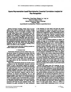
Figure 3: Approximation results using 20 uniform training data (a) Sparse approximation using sine 1 = δα∗i (− + Ei − Rii δα∗i ) + δα∗i δαi Rii kernels (b) RKHS analytic solution with RBF ker2 nels (c) Sparse approximation using RBF kernels 1 +δαi (− − Ei − Rii δαi ), (23) 2

where the elements of matrix R and the scalars Ei are defined as shown in the algorithm. With some lies within the model space being considered. The additional analysis which is omitted for brevity, we reproducing kernel of this space can be written as can show that this cost function monotonically de5  creases to a minimum value and converges provided (cos nx cos nx
+ sin nx sin nx
) K(x, x
) = the learning rate satisfies γ < 1/ max{i} Rii . Faster n=0  convergence can be obtained by using a data depen6 if x = x
dent learning rate like γi < 1/Rii . = (24) 11∗(x−x
) 1 x−x
/ sin 2 + 1] otherwise 2 [sin 2

6

Illustrative examples

This choice is equivalent to having a correlation operator R which spans the approximation space H. Using the analytical method of solving described in Section 4.2, we achieve perfect generalization i.e., the function is learned exactly. This is expected since we have noiseless data and the function resides in the search space. In comparison, when we sparsify the solution using the same sin kernel K(x, x
) (24), we get a parsimonious representation using 11 basis vectors with a normalised mean squared error(nMSE) of .00029 on a test data set as shown in Fig.3(a). The epsilon parameter in the sparse

In this section, we look at a synthetic regression task and compare the approximation properties of the RKHS based analytical solution against the more parsimonious sparse representation. We look at the task of approximating a function f = 4 − sin x + sin 2x − sin 3x + sin 4x − sin 5x shown in Fig.3 from a set of 20 uniformly sampled training data. First, we consider approximation using a function space spanned by H = {sin nx, cos nx}5n=0 . This ensures that the function to be approximated 5

training was set to  = 0.01. Next, we consider learning with a space spanned by RBF kernels with reproducing kernels


K(x, x ) = e

x−x
2 /2σ2

,

[4] C. Cortes and V. Vapnik. Support vector networks. Machine Learning, 20:273–297, 1995. [5] D.J. Field. Relation between the statistics of natural images and the response properties of cortical cells. Journal of Optical Society Am., 4:2379–2394, 1987.

(25)

where σ is the variance parameter of the kernel which we set here to a value of σ = 0.5. Hence, in this case the function we are trying to approximate does not strictly lie in the search space. The result of learning with 20 points using the RKHS analytic method is shown in Fig.3(b) resulting in an nMSE=0.00092. Using the sparseness constraint in this function space leads to an approximation with 12 basis vectors and an nMSE of 0.0361 as shown in Fig.3(c). Here, an  = 0.2 was used. The tradeoff between accuracy and degree of sparseness can be controlled by varying the thickness of the -tube.

7

[6] F. Girosi. An equivalence between sparse approximation and support vector machines. Neural Computation, 10(6):1455–1480, 1998. [7] H. Ogawa and E. Oja. Projection filter, Wiener filter and Karhunen-Lo`eve subspaces in digital image restoration. Journal of Mathematical Analysis and Applications, 114(1):37–51, 1986. [8] P.S. Penev and J.J. Atick. Local feature analysis: A general statistical thoery for object recognition. Neural Systems, 7:477–500, 1996. [9] T. Poggio and F. Girosi. A sparse representation for function approximation. Neural Computation, 10(6):1445–1454, 1998.

Conclusion and Discussion

In this paper, we formulate the problem of learning a mapping as an inverse problem and provide analytical solutions by using an optimization criterion which exploits the apriori knowledge on the probilistic distribution of function ensembles. Although this solution is optimal from a generalization perspective, it is expensive in terms of the resources since it employs one kernel function at every training data location to represent the learned result. However, it is shown that if we choose a particular search space spanned by the correlation operator (apriori knowledge usually accessable) and enforce a sparseness constraint on the solution on the lines of Poggio and Girosi[9], the problem reduces to the same dual problem encountered in support vector regression. Here, we introduce a novel gradient descent based sequential learning algorithm to solve this dual problem for sparsification. This algorithm is simple to implement and assured of convergence within theoretically derived learning rate bounds.

[10] L. Sirovich and M. Kirby. Low dimensional procedure for characterization of human faces. Journal of Optical Society Am., 4:519–524, 1987. [11] M. Turk and A. Pentland. Eigenfaces for recognition. Journal of Cognitive Neuroscience, 3(1):71–86, 1991. [12] V. Vapnik. Statistical Learning Theory. John Wiley and Sons,Inc.,New York, 1997. [13] V. Vapnik, S.E. Golowich, and A. Smola. Support vector method for function approximation, regression estimation and signal processing. In Advances in Neural Information Processing Systems 9, pages 281–287, 1997. [14] S. Vijayakumar. Computational theory of incremental and active learning for optimal generalization. PhD thesis, Tokyo Institute of Technology, 1998.

References

[15] S. Vijayakumar and H. Ogawa. RKHS based functional analysis for exact incremental learning. Neurocomputing: Special Issue on Theoretical analysis of real valued function classes, [2] N. Aronszajn. Theory of reproducing kernels. 1999. (in press). Trans. Amer. Math. Soc., 68:337–404, 1950. [16] S. Vijayakumar and S. Wu. Sequential support [3] S. Chen, D. Donoho, and M. Saunders. Atomic vector classifiers and regression. In Proceeddecomposition by basis pursuit. Technical Reings, Soft Computing ’99 (SOCO’99), 1999. port 479, Dept. of Statistics, Stanford University, 1995. [1] A. Albert. Regression and the Moore-Penrose Pseudoinverse. Academic Press, 1972.

6