A Graphical Environment for the Design of Concurrent Real-Time

A Graphical Environment for the Design of Concurrent Real-Time Systems L. E. MOSER, Y. S. RAMAKRISHNA, G. KUTTY, P. M. MELLIAR-SMITH, and L. K. DILLON University of California, Santa Barbara

Concurrent real-time systems are among the most difficult systems to design because of the many possible interleavings of events and because of the timing requirements that must be satisfied. We have developed a graphical environment based on Real-Time Graphical Interval Logic (RTGIL) for specifying and reasoning about the designs of concurrent real-time systems. Specifications in the logic have an intuitive graphical representation that resembles the timing diagrams drawn by software and hardware engineers, with real-time constraints that bound the durations of intervals. The syntax-directed editor of the RTGIL environment enables the user to compose and edit graphical formulas on a workstation display; the automated theorem prover mechanically checks the validity of proofs in the logic; and the database and proof manager tracks proof dependencies and allows formulas to be stored and retrieved. This article describes the logic, methodology, and tools that comprise the prototype RTGIL environment and illustrates the use of the environment with an example application. Categories and Subject Descriptors: C.3 [Computer Systems Organization]: Special-Purpose and Application-Based Systems—real-time systems; D.2.1 [Software Engineering]: Requirements/Specifications—methodologies; tools; D.2.2 [Software Engineering]: Tools and Techniques—computer-aided software engineering; user interfaces; D.2.10 [Software Engineering]: Design—methodologies; representation; F.4.1 [Mathematical Logic and Formal Languages]: Mathematical Logic—mechanical theorem proving; F.4.3 [Mathematical Logic and Formal Languages]: Formal Languages—decision problems General Terms: Design, Verification Additional Key Words and Phrases: Automated deduction, concurrent systems, formal specification and verification, graphical user interface, real-time systems, temporal logic

This research was supported in part by NSF/DARPA grant CCR-9014382 under the Formal Methods in Software Engineering Program. Authors’ addresses: L. E. Moser and P. M. Melliar-Smith, Department of Electrical and Computer Engineering, University of California, Santa Barbara, CA 93106; Y. S. Ramakrishna, Computer Science Department, State University of New York, Stony Brook, NY 11794; G. Kutty Mathew, G. E. Medical Systems, P.O. Box 414, MC: W-657, Milwaukee, WI 53201; L. K. Dillon, Department of Computer Science, University of California, Santa Barbara, CA 93106. Permission to make digital / hard copy of part or all of this work for personal or classroom use is granted without fee provided that the copies are not made or distributed for profit or commercial advantage, the copyright notice, the title of the publication, and its date appear, and notice is given that copying is by permission of the ACM, Inc. To copy otherwise, to republish, to post on servers, or to redistribute to lists, requires prior specific permission and / or a fee. © 1997 ACM 1049-331X/97/0100 –0031 $03.50 ACM Transactions on Software Engineering and Methodology, Vol. 6, No. 1, January 1997, Pages 31–79.

32

•

L. E. Moser et al.

1. INTRODUCTION Designing a concurrent real-time system is an extremely difficult and challenging task. The complexity of the task stems from the large number of different possible executions of the system due to the different orderings or interleavings of concurrent events and the variability of real-time durations. Interactions between causal dependencies and real-time durations preclude reasoning about each of them separately, and thus render the task more difficult than for sequential or concurrent systems. These difficulties, and the importance of concurrent real-time systems in critical real-world applications, necessitate continued research into methodologies and tools for specifying and reasoning about the designs of such systems. Temporal logic is an appropriate formalism for reasoning about the relative ordering of events in a concurrent system [Manna and Pnueli 1992]. However, system designers have found it difficult to reason in temporal logic and to relate temporal logic to their software and hardware designs. The textual representation of temporal logic has contributed in part to these difficulties and has discouraged the use of temporal logic in industrial applications. The real-time characteristics of industrial applications have contributed further to these difficulties. Software and hardware engineers often employ graphical representations, such as timing diagrams, data flow graphs, state machines, and dependence graphs to describe properties of the systems they design [Fisler 1996; Harel et al. 1990; Schlo¨r and Damm 1993]. Such graphical representations can capture and communicate the designer’s intuitive understanding of a system. Research [Koedinger and Anderson 1990] has indicated that graphical representations do indeed facilitate human comprehension and reasoning. However, the graphical representations used by system designers often are informal and lack a well-defined meaning. To enable software and hardware engineers to describe and reason about concurrent real-time systems with greater ease and rigor, we have developed a temporal logic, called Real-Time Graphical Interval Logic (RTGIL), and a graphical environment to support its use. RTGIL employs the natural graphical representation of the time line to represent events, and intervals between events, within an execution of a system. Specifications in RTGIL resemble the “back-of-the-envelope” timing diagrams drawn by system designers and are intended to match the user’s intuitive way of thinking about the problem domain. Nevertheless, RTGIL has a rigorously defined syntax and semantics. RTGIL is a propositional interval temporal logic that is interpreted over a dense time line and is decidable. Interpretation over a dense time line simplifies the expression of real-time properties and the task of hierarchical verification. Decidability provides greater predictability for the user of verification tools based on the logic. As a propositional logic, RTGIL is not intended to be free-standing. Rather, it is intended as a temporal logic component of a more comprehensive verification system, such as EHDM ACM Transactions on Software Engineering and Methodology, Vol. 6, No. 1, January 1997.

Design of Concurrent Real-Time Systems

•

33

[Crow et al. 1990] or PVS [Owre et al. 1995], that provides support for multiple theories and quantification. The RTGIL environment that we have developed employs a propertytheoretic or axiomatic approach to design, specification, and verification of concurrent real-time systems. Like automated theorem proving in general, mechanical verification of properties of concurrent real-time systems is inherently complex. Our approach to controlling that complexity exploits a symbiotic relationship between the human and the theorem prover. The user engages in the creative activity of devising the specifications that are the axioms of a theory for the system being modeled. Working in that theory and the underlying logic, the human creates theorems, lemmas, and proofs to demonstrate that the system defined by the concrete specifications satisfies the requirements imposed by the abstract specifications. The RTGIL environment provides mechanical support, routine reasoning and checking, attention to detail, completeness, and accuracy. The advantage of a property-theoretic approach is that it is possible to break up a complex proof into small proof steps, each of which can be understood by the human and can be checked by the mechanical theorem prover. The disadvantage is that substantial human time and effort are required. An important aspect of the RTGIL environment is that the user sees nothing of, and does not need to know anything about, the internal representations and mechanisms of the environment. All input is supplied graphically, and all output is returned to the user in the same graphical representation. The RTGIL theorem prover is based on a decision procedure, which obviates the need for a detailed understanding of its internal mechanisms and which provides predictability. Experience has shown that, without rigorous mechanical checking, it is difficult for designers to write specifications and to make correct inferences about those specifications. Inevitably they make mistakes. The RTGIL environment helps to find such errors. If an attempted proof is not valid, the environment displays a counterexample in a graphical representation that is easy for the user to understand and to relate to the graphical representation of the failed proof attempt. The software architecture of the RTGIL environment is shown in Figure 1. The graphical editor of the RTGIL environment enables the user to construct graphical formulas on a workstation display and checks whether those formulas are syntactically correct. The automated theorem prover consists of a tableau-based decision procedure that checks the validity of proofs in the logic and a counterexample generator that produces counterexamples to failed proof attempts. The database and proof manager tracks proof dependencies and allows graphical formulas to be stored and retrieved. 2. REAL-TIME GRAPHICAL INTERVAL LOGIC The basic concepts of RTGIL are presented below. Appendix A provides a formal abstract syntax and model-theoretic semantics for the logic. The decidability of RTGIL is established in Ramakrishna et al. [1996b] by means of ACM Transactions on Software Engineering and Methodology, Vol. 6, No. 1, January 1997.

34

•

L. E. Moser et al.

Fig. 1. The software architecture of the RTGIL environment includes a graphical editor, an automated theorem prover, and a database and proof manager. Rectangles in the diagram represent program modules, and ovals represent data structures through which information is communicated between program modules in the directions indicated by the arrows.

an automata-theoretic decision procedure; an axiomatization is currently being developed. Further examples of RTGIL formulas appear throughout the remainder of the article, in particular in Section 6 and Appendix B, where specifications and proofs for an input-output system are presented. Formulas in pure temporal logic involve invariants, eventualities, and order constraints, allowing us to express safety and liveness properties, while making no reference to time. However, the correctness of real systems often also depends critically upon the real time between events within the system. Much of the elegance of temporal logics is that the value of time and the quantification over time are hidden by the logic, facilitating automatic processing by decision procedures. We preserve this characteristic in RTGIL by defining intervals over which properties are asserted to hold and by defining bounds on the durations of intervals. This allows us to express time-bounded safety and liveness properties. In RTGIL an interval represents a trace of states of a computation, defined on a dense time line, rather than on a discrete time line as in many ACM Transactions on Software Engineering and Methodology, Vol. 6, No. 1, January 1997.


•

35

other temporal logics. These traces, or models, are required to be right continuous and finitely variable (see Appendix A for the formal definitions). Right continuity forces each primitive proposition to hold its value for a nonzero duration. It thus excludes the occurrence of instantaneous states and captures our intuition that any state of the system must persist for a measurable amount of time; we do not, however, impose any a priori lower bound on those durations. Finite variability ensures that there are only finitely many state changes in any bounded interval of time. It thus precludes the existence of Zeno runs in which the system undergoes infinitely many changes before any finite point in time. Zeno runs and instantaneous states cause problems for hierarchical verification [Abadi and Lamport 1994], similar to those caused by the next time operator of temporal logics interpreted over a discrete time line. Finite variability ensures that any specification that attempts to define Zeno behavior is inconsistent and thus unsatisfiable. It is, of course, essential to show that a specification is satisfiable, since anything can be deduced from an inconsistent specification. Unfortunately, a direct demonstration that a specification is satisfiable may be computationally infeasible. However, if we can exhibit a concrete model, possibly derived from an implementation, and can demonstrate that the model is non-Zeno and satisfies the specification, then we have also demonstrated the non-Zenoness of the specification. 2.1 Graphical Constructs of RTGIL In RTGIL the progression of states of a computation in time is shown using a horizontal time line. An interval is represented by a segment of the time line and is delimited by two states, which correspond to its left and right endpoints. Lower and upper bounds can be placed on the duration of an interval. Formulas in RTGIL are read from top to bottom and from left to right, starting with the topmost interval which represents an entire computation. Formulas can be combined using standard logical infix operators laid out vertically. In vertical layout a conjunction is indicated by stacking the formulas one below the other without the conjunction operator. Braces are used to disambiguate formulas. Syntactically, an interval is defined by two search patterns, one for each of its endpoints. Each search pattern is a sequence of one or more searches. A search in a search pattern begins at the start of the context, or at the state located by the previous search in the sequence, and locates the next state in the future (to the right) at which its target formula holds. The last search in a search pattern locates the state that corresponds to the endpoint of the interval defined by the search pattern. An interval is half-open in that it includes its left endpoint, but not its right endpoint. As shown in the formulas below, searches are represented by dashed horizontal line segments with arrowheads, search patterns by a sequence of such line segments, and intervals by solid horizontal line segments, delimited by [ and ). In these formulas f, g, and h can be replaced by any RTGIL ACM Transactions on Software Engineering and Methodology, Vol. 6, No. 1, January 1997.

36

•

L. E. Moser et al.

formula. Once an interval has been defined, properties can be asserted to hold on the interval. The different types of properties are given below. Initial Property. To assert that a formula holds at the first state of an interval, the formula is drawn left-justified below the left endpoint of the interval. For example,

asserts that h holds at the first state of the interval that begins with the first state at which f holds and ends just prior to the next state at which g holds. Henceforth Property. To express an invariant (henceforth) property that holds throughout an interval, the formula that is asserted to be invariant is positioned below the interval and is indented to the right of the bracket that delimits its start. For example,

asserts that h holds at every state of the interval that begins with the first state at which f holds and extends up to, but does not include, the next state at which g holds. Temporal expressions that are invariant over the entire computation are indented beneath the topmost interval. Eventuality Property. To express an eventuality property, a diamond { is placed on the interval, with the eventuality property left-justified below the diamond. For example,

asserts that h holds at some state of the interval that begins with the first state at which f holds and extends up to, but does not include, the next state at which g holds. Weak versus Strong Searches and Intervals. If the target formula of a search does not hold at any state in the future of the state at which the ACM Transactions on Software Engineering and Methodology, Vol. 6, No. 1, January 1997.


•

37

search begins, the search to the formula fails. This differs from a search without a target formula, i.e., a search to the end of the context, which always succeeds. If either of the searches for the left or right endpoints of an interval fails, or if the state located by the search for the right endpoint coincides with the state located by the search for the left endpoint, the interval cannot be constructed. If the interval cannot be constructed, the interval formula holds vacuously. The single-arrow searches and single-line intervals in the previous examples are referred to as weak searches and weak intervals, respectively. The logic also provides strong searches and strong intervals. The strong search, denoted by a dashed line segment with double arrowheads as, for example, in

expresses the requirement that the search to g must not fail. More specifically, it requires that the search to g must succeed unless the weak search to f fails. The strong interval, denoted by a double solid line, in the following example

requires that the interval is nonempty, provided that the searches to f and g do not fail. In effect, it means that following the first occurrence of f, if any, the first future occurrence of g, if any, must be in the strict future; thus, a nonempty interval is created. Real-Time Duration Constraints. RTGIL imposes real-time bounds on the durations of intervals using the len predicate. For example,

asserts that the duration of the indicated interval, if it can be constructed, is greater than d time units and less than or equal to D time units, where d and D represent nonnegative rational constants or ` (represented as inf ACM Transactions on Software Engineering and Methodology, Vol. 6, No. 1, January 1997.

38

•

L. E. Moser et al.

in the RTGIL environment). This construct appears to suffice for describing most real-time constraints directly and easily, and it disallows the construction of undesired expressions in which time is manipulated inappropriately. As the above formulas indicate, RTGIL only admits forward searches. We have considered the addition of backward searches into the logic, but this allows the chop operator [Harel et al. 1982] to be expressed succinctly in the logic, thus rendering its decision problem nonelementary.1 To constrain the cost of theorem proving, we have intentionally restricted the logic to forward searches. Like most other real-time temporal logics, RTGIL expresses relative timing constraints rather than absolute times. 2.2 Comparison with GIL and PTL RTGIL provides the capability of expressing real-time properties, which distinguishes it from other logics such as Graphical Interval Logic (GIL) [Dillon et al. 1994] and the well-studied Propositional Temporal Logic (PTL) [Manna and Pnueli 1992]. GIL is, in fact, equivalent in expressiveness to PTL without the next operator [Kutty et al. 1995]. Although the graphical syntax of RTGIL is similar to that of GIL, the underlying model-theoretic semantics are different. Formulas in RTGIL are interpreted over a dense time line (the nonnegative reals), whereas formulas in GIL and PTL are interpreted over a discrete time line (the nonnegative integers). GIL and PTL have no capability for reasoning about real time, although real-time extensions of PTL do exist (see Section 7). The interval constructs of RTGIL, and GIL, allow more succinct and understandable statements of temporal properties than the until construct of PTL. Consider, for example, the following formula. First note that the start of the search is indented below the outer context interval, which indicates that it is an invariant property. The left endpoint of the interval is located by first searching to a state at which ¬ q holds and from there to a state at which q holds. The right endpoint of the interval is located similarly, starting from the left endpoint of the interval. The { on the interval, delimited by these endpoints, indicates that there exists a state within the interval at which p holds.

1

In other words, the worst-case complexity of the decision procedure is a stack of powers of 2, where the number of exponentiations is not bounded above by any constant.

ACM Transactions on Software Engineering and Methodology, Vol. 6, No. 1, January 1997.


•

39

This formula expresses the property that, between every pair of states at which a proposition q commences to hold, there is a state at which a proposition p holds. In PTL this property is expressed by the formula

h ~ ¬qf¬qU ~ q∧ ~ qUp∨qU ~ ¬qU ~ p∧¬q !!!!! where h is the henceforth operator, and U is the weak until operator. Although no real-time constraints appear in this example, even properties that can be expressed in PTL can often be expressed more naturally in RTGIL. The deep nesting of until formulas in the above PTL formula makes that formula very difficult for most software and hardware engineers to read and understand. 2.3 Hierarchical Abstraction, Composition, and Refinement In RTGIL, as well as in other logics [Abadi and Lamport 1995], composition is represented by the conjunction of specifications. A primary concern when composing specifications is that the set of specifications may be inconsistent, i.e., their conjunction may be equivalent to false, from which anything can be demonstrated. To ensure that a set of specifications is consistent, it suffices to show that at least one model, or computation, exists for their conjunction, i.e., that the conjunction is satisfiable. For example, the two specifications

are each individually consistent, but together they are inconsistent, i.e., their conjunction is unsatisfiable. The RTGIL environment can be used to demonstrate satisfiability and thus consistency of specifications. In general, however, a demonstration of satisfiability must consider the entire set of specifications and can easily exceed the computation time and memory resources available. A demonstration of validity is easier to mechanize because it can be derived from a subset, rather than the complete set, of specifications. Methods are available [Abadi and Lamport 1995; Moser and Melliar-Smith 1995] for demonstrating consistency by a sequence of simpler demonstrations of validity, each of which can be verified mechanically with reasonable resources. These methods are based on establishing the independence, syntactically or ACM Transactions on Software Engineering and Methodology, Vol. 6, No. 1, January 1997.

40

•

L. E. Moser et al.

semantically, of sets of specifications. RTGIL is particularly suited to such demonstrations. Properties can be defined that are restricted to an interval, and specifications defining properties in disjoint intervals can readily be demonstrated to be independent. Refinement involves the elaboration of a set of abstract specifications into a set of concrete specifications. The concrete specifications typically involve propositions that are different from those of the abstract specifications. For example, the abstract specification

might be refined into the concrete specification

Here b in the abstract specification is refined into locating a state at which c is true followed by a state at which c is false, where those two states are separated by at least 10.0 time units. A logic that is interpreted over a discrete time line may present problems for refinement. A model for the abstract specification may have only one state in the interval delimited by the state at which a is true and the state at which a is false. Such a model cannot be refined into a model for the concrete specification that contains both a state at which c is true and a state at which c is false in that interval. The dense time line of RTGIL avoids such problems. Abstraction is in some sense the inverse of refinement in that it relates the propositions of the abstract specifications to those of the concrete specifications. For temporal logics, a simple functional mapping between propositions, applied in each state separately, does not suffice. Temporal abstraction involves mappings between propositions over intervals. For some applications, the intervals of the abstract specifications are necessarily different from those of the concrete specifications, as in the above example. Abstraction, composition, and refinement are often associated with hierarchical verification. In this approach, by assuming lemmas and theorems of the concrete specifications, and by exploiting the mappings between the concrete and abstract specifications, theorems are proved of the abstract ACM Transactions on Software Engineering and Methodology, Vol. 6, No. 1, January 1997.


•

41

specifications. For example, given the following mapping between the abstract and concrete specifications

and assuming that the following two properties

hold for the concrete specifications, we can demonstrate the theorem

for the abstract specifications, using the RTGIL theorem prover. This allows the verification to begin with the demonstration of simple properties of small components of the system and to build up to the demonstration of complex properties of the entire system [Moser and Melliar-Smith 1990]. 3. THE GRAPHICAL EDITOR The graphical editor of the RTGIL environment, shown in Figure 1, enables the user to construct and edit RTGIL formulas on a workstation display. It is a syntax-directed editor that uses an attribute grammar definition of RTGIL for its implementation. Syntax-directed editors [Lunney and Perrot 1988] allow only syntactically correct formulas to be constructed and are particularly appropriate for graphical languages, such as RTGIL, as they eliminate the need for parsing. ACM Transactions on Software Engineering and Methodology, Vol. 6, No. 1, January 1997.

42

•

L. E. Moser et al.

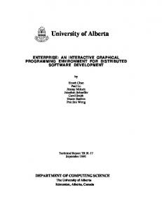
Fig. 2. The graphical user interface as it appears on a workstation display. The upper window in the background shows an attempted proof of a real-time property for the inputoutput system example in Section 6, while the lower window in the foreground shows a counterexample which demonstrates that the attempted proof is invalid. Note the lower and upper bounds on the durations of the intervals in the attempted proof and in the counterexample.

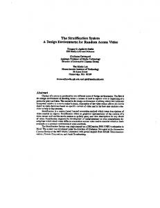
3.1 The Graphical User Interface The graphical user interface to the editor is shown in Figure 2, as it appears on a workstation display. The interface provides high-level editing operations corresponding to the constructs of RTGIL, and it provides templates containing boxes for formulas yet to be defined, as illustrated in Figure 3. The mouse allows the user to select a box or formula on the display and to highlight it. The menu-and-button interface enables the user to create and edit graphical formulas and to compose them into more complex formulas. The pull-down menus (File, Edit, Misc) at the top of the display contain commands for storing and retrieving formulas, for overriding the default layout of formulas, and for invoking the theorem prover. The buttons on the ACM Transactions on Software Engineering and Methodology, Vol. 6, No. 1, January 1997.


Fig. 3.

•

43

Editing steps taken by the user to construct an example RTGIL formula.

upper left (New, Del, Cut, Paste, etc.) provide editing operations that allow the user to create a new formula, delete a selected formula, store a selected formula in a buffer, and subsequently insert that formula in a selected box. The buttons on the lower left (Text, [—), len, etc.) are used to select an appropriate RTGIL construct to apply to the currently highlighted subformula. Scroll bars allow the user to view very large formulas. The graphical editor provides capabilities for automatically replacing formulas with other formulas, resizing formulas to suit the context length, etc. If a formula does not fit into the space allotted, an error is indicated by highlighting the formula. The user may then resize the context length or the search arrows to allow the formula to be drawn correctly. All affected subformulas of the formula are automatically resized to scale. ACM Transactions on Software Engineering and Methodology, Vol. 6, No. 1, January 1997.

44

•

L. E. Moser et al.

The editor enables the user to align corresponding points in the formulas that comprise a proof. The user can thus see how states in different formulas are ordered relative to one another, how intervals are aligned relative to each other, and how durations of intervals are related to satisfy real-time constraints. Alignment can be very helpful in constructing and debugging proofs, but has no semantic content. The graphical editor can format a formula in PostScript, suitable for printing or inclusion in a document. All of the RTGIL formulas in this article were produced directly by the graphical editor. 3.2 Implementation of the Editor The graphical editor has been implemented in Common Lisp using the Garnet graphics toolkit [Myers et al. 1990] and runs within the X windows system. The mechanisms used in the implementation of the graphical editor are described below. Graphical Objects. The graphical editor for the RTGIL environment uses the graphical object system of Garnet, which provides primitive objects such as rectangles. RTGIL formulas and other symbols required by the editor are derived directly from these primitive objects, or they are constructed by composing several of them to form a single composite object. A graphical object in Garnet is represented by a schema that consists of a set of slots and a value for each slot. The values of the slots denote relevant properties of the object. Garnet also provides aggregates for creating hierarchical structures. Attributed Syntax Trees. The graphical editor represents RTGIL formulas internally as attributed syntax trees. A syntax tree represents the structure of the corresponding RTGIL formula, and the attributes provide layout information. A node in the syntax tree represents a rectangular box, which contains the corresponding graphical formula. The attributes—left, top, width, and height— define the position of the box in the editing area. The attribute grammar relates the position of each box to the positions of the boxes for its parent and its siblings in the syntax tree. The attributed syntax trees are implemented by Garnet aggregates; the nodes in the tree are schemata, and the attribute values are kept in slots. Figure 4 shows an RTGIL formula, the structure of the formula with a rectangular box around each of its subformulas, and the structure of the formula represented by a Garnet aggregate. Attribute Evaluation. In our implementation, an attribute value of a node in the syntax tree is computed as a function of attribute values of other nodes. When an attribute value changes as the result of an editing operation, the other attribute values that depend on it must be recomputed. The consistency of the attribute values ensures that the formulas constructed using the editor are syntactically correct and appropriately positioned on the display. ACM Transactions on Software Engineering and Methodology, Vol. 6, No. 1, January 1997.


•

45

Fig. 4. An RTGIL formula, the structure of the formula with a rectangular box in thin lines around each of its subformulas, and the structure of the formula represented by a Garnet aggregate.

The constraint maintenance facilities of Garnet are used to establish the relationships between the values of slots in different schema. The value of a slot is computed only if it is actually required in the evaluation of other slots. This lazy method of evaluation results in a reasonably efficient implementation. Editing Operations. When a formula is constructed using the graphical editor, the corresponding attributed syntax tree is built incrementally. The ACM Transactions on Software Engineering and Methodology, Vol. 6, No. 1, January 1997.

46

•

L. E. Moser et al.

formulas generated by the editor initially contain boxes that are expanded into well-formed formulas during subsequent editing, as shown in Figure 3. Each expansion of a box corresponds to a production in the grammar and a corresponding operation on the attributed syntax tree. As the user performs editing operations, the attributed syntax tree is updated to reflect the edited formula. Editing operations fall into one of two categories: subtree replacement and attribute modification. Operations such as deleting a subformula and expanding a box correspond to removing a subtree from the syntax tree and replacing it with a new subtree. Routines for pruning a specified subtree and grafting a new subtree in its place are provided. Operations such as resizing an arrow or supplying an extra parenthesis do not change the underlying tree structure but only change the value of the appropriate attribute. Changing the value of an attribute in the syntax tree may, of course, require reevaluation of other attributes in the tree.

4. THE THEOREM PROVER The structure of the RTGIL theorem prover is shown in Figure 1. The decision procedure and the counterexample generator that comprise the theorem prover are described below. Theorem proving in any temporal logic that subsumes propositional calculus is at least NP-hard. Due to the greater expressiveness of most temporal logics, it is usually at least PSPACE-hard. Our approach to controlling that complexity is to have the human work closely in conjunction with the theorem prover. The RTGIL theorem prover is a satisfiability checker based on a decision procedure for RTGIL, rather than a Gentzenstyle theorem prover based on inference rules. The user, working in the theory defined by the system specifications and the underlying logic, creates theorems and proofs and submits them to the decision procedure for validation. To create and validate the proof of a theorem T, the user selects a subset of the axioms and previously proved lemmas and theorems as the premises P 1 , P 2 , . . . , P n of the proof. It is the user’s responsibility to select a set of premises sufficient to establish the theorem but small enough to keep the proof time reasonable; intermediate lemmas and theorems may be required. The graphical editor displays the proof represented by the formula P1 ∧ P2 ∧ . . . ∧ Pn f T in its graphical form, as illustrated in Figure 2. The reduction module, shown in Figure 1, converts the graphical representation of this implication into a textual representation for use by the theorem prover. The textual representation is generated by traversing the syntax tree and ignoring all attributes that are not relevant to the theorem prover, in particular the layout attributes. The Lisp S-expression so generated for the implication is then submitted to the theorem prover for refutation. ACM Transactions on Software Engineering and Methodology, Vol. 6, No. 1, January 1997.


•

47

The theorem prover invokes the decision procedure on the negation of the implication. If the decision procedure finds a satisfying model for the negated implication the attempted proof fails, and the generated model is a counterexample to the attempted proof. In this case we refer to the attempted proof as an “invalid proof.” If no such satisfying model exists the implication is valid, and the attempted proof succeeds. The theorem prover exploits the fact that RTGIL, as a propositional logic, is decidable [Ramakrishna et al. 1996b]. Quantification is, of course, necessary to specify and verify complex properties of concurrent real-time systems. We plan to integrate the theorem prover into a verification environment, such as EHDM [Crow et al. 1990] or PVS [Owre et al. 1995], which includes decision procedures for other theories, as well as a Skolemizer and facilities for naming, typechecking, and modularization. In such a verification environment, existentially quantified formulas are reduced to ground terms, which the decision procedures can handle, by having the user supply instances of the existentially quantified variables. For RTGIL, the time variable never needs to be instantiated, since it is hidden from the user. 4.1 The Decision Procedure As for most temporal logics, a decision procedure for RTGIL may be given as an automata-theoretic method [Ramakrishna et al. 1996b]. In that approach, the satisfiability problem for the logic is reduced to the emptiness problem for the corresponding automaton. For typical formulas, the automata-theoretic method is unnecessarily inefficient in both time and space. The decision procedure that we have implemented is therefore a tableau-theoretic method. It is an extension of the conventional tableautheoretic method [Wolper 1985], deriving its novelty from the timed tableau and region tableau that it employs to handle real-time duration constraints. A tableau for a formula f may be viewed as a directed graph in which each node represents a set of states, and each edge represents a set of transitions between states in the source and target nodes. Each node is labeled by a set of subformulas of the formula f that hold in all of the states represented by that node. The formulas in this set give rise to a set of propositional requirements on the states represented by the current node and a set of requirements for the future. The latter constrains the choice of nodes that can be successors of the current node by constraining the truth values of both primitive propositions and temporal formulas in future states. An edge connects two nodes in the tableau if and only if, from every state represented by the first node, a transition is possible to some state represented by the second node. The representation of a set of states by a node does not actually enumerate those states, but rather enumerates the subformulas that hold at those states. By clustering states and transitions in this manner, the tableau-theoretic method typically achieves better time and space efficiency than the automata-theoretic method. ACM Transactions on Software Engineering and Methodology, Vol. 6, No. 1, January 1997.

48

•

L. E. Moser et al.

For each node in the tableau that contains an eventuality formula, the procedure checks for the existence of a path in the tableau such that the eventuality is satisfied at some point in the future of that node. Nodes containing eventualities that are not satisfied are pruned from the tableau. If the procedure terminates by pruning all of the initial nodes from the tableau, then the formula is unsatisfiable. Otherwise, a satisfying model for the formula can be extracted from the tableau, in the form of an infinite path through the tableau in which all eventualities are satisfied, by projecting the set of formulas labeling each node of the path down to the primitive propositions and their negations. A detailed formal description of the tableau method underlying the theorem prover is beyond the scope of this article, requiring the introduction of much additional technical machinery [Ramakrishna et al. 1996a; 1996b]. Here we confine ourselves to a high-level description using a simple example to illustrate the major steps of the algorithm, which involve construction of an untimed tableau, a timed tableau, and a region tableau. Suppose then that we wish to check the satisfiability of the formula f given by

which is represented textually as v3 ¬a, 3ai 3Bb))len (1.0, 2.0]. The Untimed Tableau Construction. The first part of the algorithm constructs the initial untimed tableau corresponding to the formula f. We start, as illustrated in Figure 5, with an initial node containing f. At every step, we check the requirements imposed by the set of formulas that comprise the current node and abandon a node if it leads to a propositional inconsistency. For the initial node, the requirements on the future depend on whether ¬a, the target of the first search, holds at present. This leads to a case split, in which the initial node is split into two nodes, corresponding to { f, a} and to { f, ¬ a}. The formula ¬a which forced this choice is called a reductor of the formula f. Consider the node containing f and ¬a in Figure 5. Since the search to ¬a is already satisfied, we require that f 1 5 v3ai3Bb))len(1.0, 2.0] should also hold at the current state. We say in this case that ¬a reduces f to f 1 . The next possible choice for a reduction is based on the target of the next search in f 1 , namely a. But this choice is precluded, since ¬a holds at the current state. Thus, f 1 is irreducible, and the requirement that f 1 must hold at the current state translates into a requirement that it must hold in the immediate future. The node N 2 is thus a completed node, and we create a successor node to which we propagate the requirement f 1 . ACM Transactions on Software Engineering and Methodology, Vol. 6, No. 1, January 1997.


•

49

Fig. 5. Construction of the initial untimed tableau by reduction and choice within nodes (shown by means of thin lines) and propagation across nodes (shown by means of thick arrows).

No further choices or reductions are forced in N 1 , which likewise becomes a completed node, and its requirement f is propagated into its future. When the new node representing the successor of N 1 is reduced, it is split into two nodes containing precisely the same sets of formulas as N 1 and N 2 . Consequently, we do not create new nodes for the successors of N 1 but, rather, insert edges to indicate that N 1 and N 2 are the possible successors of N 1 . Proceeding in this manner, we obtain the initial untimed tableau, shown in Figure 6 with formula abbreviations in Table I, which is the graph consisting of the completed nodes and the edges that have been determined. It is not difficult to see that the expansion of the tableau must terminate, since all of the formulas introduced during the process are subformulas of the original formula. (Here we use subformula in a semantic sense, somewhat different from the usual syntactic notion of subformula. See Ramakrishna et al. [1996a; 1996b] for the precise technical meaning.) The extension of a branch can be terminated as soon as a previously encountered set of formulas is obtained. While the initial untimed tableau handles untimed safety properties correctly, it does not, in general, handle liveness properties correctly, because it may contain paths that postpone forever the fulfillment of eventualities. An example eventuality is the formula f 7 5 ¬[3b u 3)false, which requires b to hold at some state in the future. In general, if there is a node in the tableau containing a formula of the form ¬[3g u 3)false, which requires the formula g to hold at some future state, but for which there is no reachable node containing g, then that node and its associated edges are removed from the tableau. This pruning of the tableau is repeated, using an ordinary depth-first-search reachability check, until no further nodes can be removed. In the worst case, the cost of this pruning is ACM Transactions on Software Engineering and Methodology, Vol. 6, No. 1, January 1997.

50

•

L. E. Moser et al.

Fig. 6. Construction of the initial untimed tableau for f. See Table I for the abbreviations f 1 through f 7 .

proportional to the product of the number of occurrences of eventuality formulas in the tableau and the total number of nodes in the tableau. From Untimed to Timed Tableau. The tableau obtained at the end of the previous stage is called an untimed tableau because, although it handles non-real-time properties correctly, it does not yet have any quantitative notion of time and, thus, cannot check the satisfaction of real-time constraints. These constraints are already present in the nodes of the untimed tableau as formulas of the form (len(0, D] and (¬len(0, D]. (Note that the formula (len(d 1 , d 2 ] is equivalent to (¬len(0, d 1 ] ∧(len(0, d 2 ] by the semantics of RTGIL.) The decision procedure uses this information in the nodes of the untimed tableau to build a timed tableau by introducing timers to keep track of the time elapsed between events in the tableau. ACM Transactions on Software Engineering and Methodology, Vol. 6, No. 1, January 1997.

Design of Concurrent Real-Time Systems Table I.

•

51

Abbreviations for Formulas used in the Example

Consider now, as an example, the node N 4 containing the formula f 5 5 [2 u 3b)len(0.0, 2.0]. We start a timer T 1 on transitioning into the node and subsequently check, whenever b next becomes true (i.e., on transitioning into node N 8 ), that the timer satisfies T 1 # 2.0. Similarly, for handling lower bounds on interval durations, such as those required by the formula f 3 5[2 u 3b)¬len(0.0, 1.0], we wait until the next state when the formula f 4 5 [2 u 3b)len(0.0, 1.0] becomes true and, at this transition, activate a timer T 2 . (Observe that for f 3 to hold now, f 4 must hold before b becomes true.) At the first subsequent time when b becomes true, we check that T 2 5 1.0. A timer is deactivated as soon as the right endpoint of the interval that it is timing has been encountered. In this manner, we obtain a timed tableau in which a set of active timers is associated with each node and in which a set of timer actions (activation and deactivation) and timer tests is associated with each edge. The timer augmentation details for the example are listed in Tables II and III. The Region Tableau and Emptiness Checking. Having obtained the timed tableau, we now check that it contains a trace that respects not only the liveness conditions, but also the real-time constraints imposed by the timers. We use a variation of Dill’s algorithm [Dill et al. 1989] to check whether such a trace exists. Consider, for instance, the transition that takes us from node N 2 to node N 4 , while activating the timer T 1 . The value of T 1 in node N 4 satisfies the trivial condition {0.0 # T 1 }. Such a set of constraints on the active timers associated with a node is called its timer region. Consider now an outgoing transition, say (N 4 , N 6 ), which carries the timer condition T 1 # 2.0. By our model-theoretic assumption, each state has a nonzero duration, so T 1 is strictly greater than 0.0 when an outgoing transition is taken. The transition (N 4 , N 6 ) can be taken only if there is a nonempty intersection between the region {0.0 , T 1 } associated with the source node and the region {T 1 # 2.0} defined by the transition constraints. Since this is so, the transition can be taken. In the process of taking this transition, we must also activate the timer T 2 . For the node N 6 , the timer values must, therefore, satisfy the ACM Transactions on Software Engineering and Methodology, Vol. 6, No. 1, January 1997.

52

•

L. E. Moser et al. Table II.

Table III.

Active Timers Associated with Nodes in the Timed Tableau (nodes with no active clocks have been omitted)

Timer Conditions and Actions Associated with Transitions in the Timed Tableau (edges with no timer actions and no timer conditions have been omitted)

following set of conditions:

$ 0.0 , T 1 ,

0.0 # T 2 ,

T2 , T1 ,

T 1 2 T 2 # 2.0 %

This set of conditions defines the timer region associated with N 6 , when entering it from N 4 as above. Observe that there is another path by which it is possible to enter N 6 , and this path might associate a different region with N 6 , requiring replication of this node. However, for our simple example, both paths produce the same region for N 6 , and no replication is required. In our construction, we must also delete any transition that yields an empty intersection between the previous region and the region defined by conditions of the next transition. We call the graph obtained after the above steps have been completed a region tableau. Dill et al. [1989] have shown that there is an effective and, in fact, canonical representation of regions using so-called difference bounds matrices and that the construction of this graph terminates when rational numbers are used for timer conditions. The region tableau for our simple example, however, contains the same nodes and edges as the timed tableau; the regions associated with each node are listed in Table IV. Since building the region tableau may eliminate paths from the untimed tableau, a further round of tableau pruning is needed to ensure that eventualities are fulfilled. The original formula f is satisfiable if and only if at the end of this step an initial node of the tableau remains. In our example, no transition is eliminated during the construction of the region tableau, and this check need not be repeated. It is easy to extract a satisfying model for the formula f from the final tableau. ACM Transactions on Software Engineering and Methodology, Vol. 6, No. 1, January 1997.

Design of Concurrent Real-Time Systems Table IV.

•

53

Regions Associated with the Nodes in the Region Tableau (nodes with no active clocks have been omitted)

Efficiency Considerations. Although we have described our construction in three distinct steps for expositional ease, it is more efficient to construct the region tableau on-the-fly while maintaining its strongly connected components. We define a bottom strongly connected component to be a strongly connected component that does not lead to any other strongly connected component of the graph. As soon as a bottom strongly connected component of the region tableau is constructed that is not self-fulfilling (i.e., does not satisfy all of its eventualities), that component can immediately be deleted from the tableau, thus saving memory space, which is a critical resource. If a bottom strongly connected component is constructed that is self-fulfilling, the procedure terminates with the answer that the formula is satisfiable, and a satisfying model for the formula can then be extracted. The advantages of this on-the-fly approach are that the space requirements are smaller and that the entire tableau need not be constructed before a satisfying model is found. The disadvantage is that the procedure might be slower because some bottom strongly connected components may have to be recomputed each time they are reached by different paths. This enhancement to the decision procedure causes invalid proofs to be identified substantially more quickly, although valid proofs may take slightly longer to verify. In most verification contexts, this is an advantageous trade-off. In Ramakrishna et al. [1996b] we showed the elementary decidability of RTGIL by reducing its decision problem to the emptiness problem of timed Bu¨chi automata [Alur and Dill 1990]. The decision procedure is in EXPSPACE. For a formula with n propositional and temporal terms, depth k of interval nesting, and size t of the binary encoding of the timing constants in the formula, we obtain a DEXPTIME(n 2k z k z log n 1 t z log t) decision procedure. This complexity is at least as good as that for any other decidable dense real-time temporal logic known to us. In practice, the decision procedure is quite well matched to the human user. A proof that is too complicated to be decided in a reasonable time by the decision procedure is also sufficiently complicated that the human is likely to have made mistakes while devising it. 4.2 The Counterexample Generator If the decision procedure determines that an attempted proof is invalid, the user can invoke the counterexample generator to produce a counterexample ACM Transactions on Software Engineering and Methodology, Vol. 6, No. 1, January 1997.

54

•

L. E. Moser et al.

to the invalid proof. A model satisfying the negation of the implication representing the proof is then extracted from the tableau. This model is a counterexample to the invalid proof. The counterexample is displayed in an auxiliary window (shown in Figure 2) as a sequence of contiguous intervals of a computation, represented as a sequence of rectangles, with a list of values of the predicates in each interval and with real-time constraints below the intervals. A timing diagram is also shown if the user selects that option. By associating the targets of the searches in the formulas of the proof with the intervals in the sequence at which the predicates become true or false, or the points in the timing diagram at which the signals rise or fall, the user can more readily discover the fallacy in the reasoning and correct it (see the example in Section 6.3). In addition to checking formulas for validity, the user can also invoke the decision procedure to check a formula for satisfiability. The decision procedure then tries to find a satisfying model for the formula. If such a satisfying model exists, the user can invoke the counterexample generator to extract a model from the tableau and to display it. Satisfiability checking enables the user to determine whether a set of specifications is consistent. 5. THE DATABASE AND PROOF MANAGER The RTGIL environment also includes a simple database and proof manager, shown in Figure 1 and described below. The most interesting issue here is how the graphical formulas of RTGIL are stored efficiently. 5.1 The Database In the RTGIL database, formulas are stored on disk in Unix files. Several formulas can be stored in the same file by associating a unique name with each of them; these names are used for subsequent retrieval of formulas. The user can invoke the editor to display the names of the formulas in a file and to load, add, or delete a formula to, or from, a file. A textual representation is used to store RTGIL formulas in a file, because the graphical representation would require an excessive amount of storage. This textual representation is different from that used by the theorem prover, since now it is necessary to store layout attributes needed to reconstruct the graphical representation of the formulas. A formula is stored in the form of Lisp function calls (with appropriate arguments) to specific functions that reconstruct the attributed syntax tree. These are precisely the functions that are invoked by the syntaxdirected editor during the construction of the formula. This method of storage allows the formula to be easily reconstructed and is more space efficient than storing the attributed syntax tree itself. 5.2 The Proof Manager The RTGIL proof manager aids the construction of large proofs. A specially designated file is used to store information about proofs that have been ACM Transactions on Software Engineering and Methodology, Vol. 6, No. 1, January 1997.


Fig. 7.

•

55

An input-output system based on a four-phase handshaking protocol.

successfully validated by the theorem prover in the current verification effort. For each formula in a file, the user can invoke the proof manager to determine if a proof for the formula already exists and to list the premises of the proof. If a proof does not exist, the editor interactively queries the user for the premises of the proof. The user then lists the appropriate specifications and lemmas by name. When the user has finished supplying the premises, the editor displays the graphical formula that represents the proof. The theorem prover immediately proceeds to check the validity of this formula. The user can also construct a proof directly and then invoke the theorem prover to check whether or not the proof is valid. If an attempted proof succeeds, the proof dependency file is updated to include information about the proof and the time at which it was performed. This information is used to ensure that the proof is up-to-date by checking that neither the theorem nor any of the premises of the proof has been modified since the time of the proof. The proof manager also detects circularities in a proof and ensures that no cycles are introduced into the proof dependency graph. A prove-all option allows the user to proof check the entire proof dependency graph above a specific formula. This option rechecks the validity of those proofs that are out-of-date, using the last modification times of the formulas involved.

6. AN EXAMPLE APPLICATION We now present an example application of the use of the RTGIL environment for reasoning about real-time properties of an input-output system. The input-output system is based on a four-phase handshaking protocol and is widely used in industrial control computers, in embedded computers, and in personal computers. In such a master/slave system, the input and output are controlled by the processor which selects the device to, or from, which data are to be transferred, as Figure 7 illustrates. In this example, we only show the input from the device to the processor and present specifications for a single device. Generalizations to both input and output, and to multiple devices, are straightforward. ACM Transactions on Software Engineering and Methodology, Vol. 6, No. 1, January 1997.

56

•

L. E. Moser et al.

6.1 The Input-Output System The input-output system involves two agents: a requester (the processor) and a responder (the device). The requester sets the following: —addr: a predicate representing the presence of address information on the address bus. —req: a boolean control signal indicating to the responder that the requester has placed address information on the address bus. The responder sets the following: —data: a predicate representing the presence of data on the data bus. —resp: a boolean control signal indicating that the responder has received the requester’s address information and that the responder has placed information on the data bus for the requester. Initially, all four signals are false. The handshaking protocol operates in four phases: (1) The requester places information on the address bus and, after a short delay, sets req to true. The delay between setting addr and setting req is intended to ensure that the information on the address bus is available to the responder before the responder detects that req has become true. (2) The responder detects that req has become true and reads the address information on the address bus. It then places the requested information on the data bus and, after a short delay, sets resp to true. (3) The requester detects that resp has become true and reads the information on the data bus. At this point, the requester knows that the responder has detected that req has become true and has read the information on the address bus. The requester then sets addr and req to false. (4) The responder detects that req has become false and knows that the requester has read the information on the data bus. The responder then sets data and resp to false. Once the requester has detected that resp has become false, the requester can restart the cycle by placing further information on the address bus. The specifications for the four-phase handshaking protocol are given in Appendix B. The relationships between these specifications and the conventional timing diagram representation of the protocol are given in Figure 8. The specifications are labeled S for the requester and R for the responder. This example illustrates significant advantages of RTGIL for specifying real-time constraints. Frequently, system designers need to express constraints on the durations of intervals between one signal and the next signal. For example, Specification S1 constrains the duration of the interval between setting addr and setting req to be between 1.0ms and 2.0ms. Another common need is to ensure that a signal, once set, remains set for a ACM Transactions on Software Engineering and Methodology, Vol. 6, No. 1, January 1997.


•

57

Fig. 8. The relationships between the specifications and the conventional timing diagram representation of the four-phase handshaking protocol for the input-output system. The specifications are labeled S for the requester and R for the responder.

certain minimum duration to prevent glitches in the logical circuitry. For example, Specification S7 requires that req must remain true for more than 10.0ms before going false again. Moreover, practical systems must react appropriately when one of the agents fails—for example, the processor must not wait forever. Consequently, Specification S7 also requires the requester to remove its req signal within 20.0ms even if no resp signal is detected. The durations of the data and resp signals are similarly constrained. The specifications become more complex when two timing constraints interact. For example, Specification S9, which requires req to become false 2.0ms to 5.0ms after resp becomes true, may conflict with Specification S1. Consequently, Specifications S8, S9, and S10 involve a three-way case split. Specification S9 represents the normal case in which resp is neither early nor late; thus, the timing of req going false is determined relative to resp becoming true, without conflicting with the constraints of Specification S7. If resp becomes true sufficiently early, Specification S8 determines the timing of req going false. If resp becomes true too late, or never becomes true, Specifications S10 determines the timing of req. This case split is not an artifact of RTGIL, but is inherent in the application and, indeed, in many other applications whose timing constraints are precisely specified. To be effective in practical applications, a real-time temporal logic must be able to express complex temporal constraints. 6.2 Proof of a Time-Bounded Recurrence Property The following theorem expresses the time-bounded recurrence property that, starting from a state at which all four signals are false, the requester having set req to true and then to false again, there exists another state at which all four signals are false and that state occurs within 17.0ms. ACM Transactions on Software Engineering and Methodology, Vol. 6, No. 1, January 1997.

58

•

L. E. Moser et al.

This property, that the system returns to a quiescent state in which it is available for the next activity within a real-time bound, is precisely the type of property that must be demonstrated for many practical applications. To add interest to the proof, we do not use Specifications R8, R9, and R10. In effect, we demonstrate that, even if the handshaking fails so that the responder does not detect req becoming false, the values of the time constants are such that all four signals indeed return to false within 17.0ms. In Appendix B we present the lemmas for the proof of the theorem. The lemmas and proofs were created by the human, using the graphical editor, and were then submitted to the theorem prover for validation. This approach to automated theorem proving, which is used in specification and verification systems such as EHDM [Crow et al. 1990] and PVS [Owre et al. 1995], has the advantage that it exploits the understanding and creativity of the human and the completeness and precision of the theorem prover. It permits mechanical theorem proving within the time and space limits of existing workstations. Proofs of Invariant Properties. Proofs involving initial properties, rather than invariant properties, are less expensive for the theorem prover and are easier for humans to understand. Since all of our specifications but one are invariant properties, we use them as initial properties to prove an initial property (Lemma L11) and then use metatheoretic reasoning to derive the invariant property expressed by the theorem. From the semantics of RTGIL, it follows that, if (hF ∧ S 0 ) f G is valid, then hF f h(S 0 f G) is valid. In the proof, we let S 0 be the initial specification, hF the remaining invariant specifications, G Lemma L11, and hT the theorem to be proved. Using the theorem prover, we then prove that h(S 0 f G) f (S 0 f hT) is valid (see Figure 11). From the semantics of RTGIL, we then have the desired result that (hF ∧ S 0 ) f hT is valid. Example Proofs. Lemmas L7 and L10 are two of the key lemmas used in the proof of the theorem. Lemma L7 establishes that the duration of the interval from req to ¬resp is bounded by 13.0ms and 27.0ms. To perform the ACM Transactions on Software Engineering and Methodology, Vol. 6, No. 1, January 1997.


•

59

Fig. 9. The proof of Lemma L7. In this proof, the bounds of 3.0ms and 7.0ms on the interval from req to resp, established by Lemma L6, are combined with the bounds of 10.0ms and 20.0ms on the interval for which resp remains true, required by Specification R7. Lemma L3 establishes that data is false when resp becomes false. Note that in Lemma L6 the strong search and the strong interval imply that resp must become true and that the interval is nonempty. This result is combined with Specification R7 which, as an invariant, is applicable whenever resp becomes true.

proof of Lemma L7, shown in Figure 9, the user first creates the formulas that comprise the proof using the graphical editor and stores them in the specification database with the names S0, L6, R7, L3, and L7. The user then invokes the theorem prover, whereupon the proof manager determines that a proof does not already exist. The graphical editor then interactively queries the user to supply the premises of the proof. The user supplies the names S0, L6, R7, and L3, and the editor automatically generates the proof in its graphical form and displays it to the user. The theorem prover then checks the validity of the proof as represented by the given implication. The proof of Lemma L7 required 31 seconds by the theorem prover on a 167MHz Sun UltraSPARC workstation. The graphical nature of RTGIL makes it easy for the user to create specifications and proofs. Consider Specification R7, illustrated in the proof of Lemma L7. The user constructed the interval from resp to ¬resp and constrained the duration of that interval to be more than 10.0ms and at most 20.0ms. The forward searching, and the local searches to the next state at which a search predicate is true, makes the logic more operational ACM Transactions on Software Engineering and Methodology, Vol. 6, No. 1, January 1997.

60

•

L. E. Moser et al.

and, therefore, easier for system designers to use. Furthermore, the realtime constraints are naturally expressed as bounds on the durations of intervals. In the proof of Lemma L7, the duration of the interval from req to resp to ¬resp and ¬data is naturally derived from the constraint on the duration of the interval from req to resp, given in Lemma L6, and the duration of the interval from resp to ¬resp, given in Specification R7. Lemma L3 determines that data is false when resp becomes false. Note how these three formulas are aligned in the proof so that the states at which resp is true and the states at which resp is false are positioned vertically. We have found that this alignment makes it easy to construct proofs, and to check them, by stepping down the formulas of the proof making certain that each specification or lemma does indeed properly match those above it. Lemma L10 concludes that either the interval from ¬req and ¬addr to addr is bounded below by 18.0ms, or else the interval contains a time at which resp and data become false, as indicated by the double arrowhead. The proof of Lemma L10, shown in Figure 10, looks more complex than that of Lemma L7, but really it is just a case split, simpler than the proof of Lemma L7 and validated by the theorem prover in 16 seconds. In general, initial properties are computationally more tractable than henceforth properties, especially when those properties involve real-time constraints. Again, in constructing the proof of Lemma L10, the user first stores the formulas that comprise the proof in the specification database. On invoking the theorem prover for Lemma L10, the user finds that no proof exists and then supplies the graphical editor with the names S0, S12, S13, S14, L2, and L5 as the premises of the proof. The editor then assembles the proof and displays it to the user in its graphical form, whereupon the theorem prover checks the validity of the proof. Finally, in Figure 11 we exhibit the proof which yields the theorem that expresses the time-bounded recurrence property. This proof required 27 seconds by the theorem prover. To show that the theorem follows from the original specifications, we apply the metatheoretic reasoning described above. Construction of the specifications and proofs for the four-phase handshaking protocol example took about five person-days spread over a month. Multiple iterations were required to achieve appropriate specifications. 6.3 A Counterexample Model In the event that an attempted proof is invalid, the user can request the counterexample generator to extract a counterexample from the tableau and to display it. For example, while attempting to prove Lemma L10, the user accidentally used Lemma L3 in place of the very similar Lemma L5, resulting in an invalid proof. The user then requested the counterexample generator to provide the counterexample shown in Figure 12. We now examine the counterexample to determine why the proof failed. The only difference between Lemma L3 and Lemma L5 is the substitution ACM Transactions on Software Engineering and Methodology, Vol. 6, No. 1, January 1997.


•

61

Fig. 10. The proof of Lemma L10. In this proof, Specifications S12, S13, and S14 form a case split that determines how long a period must elapse between req becoming false and addr becoming true, depending on when resp becomes false. Lemma L10 shows that either this interval is more than 18.0ms, or else it contains a time at which resp and data become false, as indicated by the double arrowhead. Lemmas L2 and L5 show, respectively, that addr and data are false when req and resp become false.


62

•

L. E. Moser et al.

Fig. 11. This proof yields the theorem that expresses the time-bounded recurrence property. The proof employs Specification S0 and Lemma L11. To see that the theorem follows from the original specifications, we apply the metatheoretic argument of Section 6.2.

of ¬req for resp in the third search. The proof of Lemma L10 involves a case split that depends on when resp becomes false after req has become false, and on resp and data being false simultaneously, as required by both Lemma L3 and Lemma L5. However, the erroneous use of Lemma L3 in the proof allowed, at the time req became false in the third interval, resp to be false without data being false. This satisfies Specification S12 of the case split and permits the interval from ¬req to addr (the third and fourth intervals) to have a duration greater than 10.0ms. Subsequently, in the fifth interval, both resp and data become false but only when addr also becomes true, in contradiction to Lemma L10. ACM Transactions on Software Engineering and Methodology, Vol. 6, No. 1, January 1997.


•

63

Fig. 12. The top of the figure shows a sequence of contiguous intervals of a computation, represented as a sequence of rectangles, with a list of values of the predicates in the interval. If a predicate is not listed, it can have either value true or false in the interval. Below the sequence of intervals are the real-time constraints satisfied by the computation, and below them is a timing diagram for the predicates.

Comparing the sequence of intervals in the counterexample with the sequence of target states in Lemma L3, it is clear why that lemma did not achieve the desired effect and what had to be done to correct the proof. The reasoning employed in these proofs is intricate, because of the interactions between real-time constraints, non-real-time temporal (causalorder) constraints, and nontemporal logical constraints. It is best checked mechanically and exhaustively by a computer rather than by a human. In contrast, the construction of the proofs, by selection of the appropriate specifications and lemmas, is a highly skilled and creative human activity requiring considerable understanding of the application and of the reasons why particular theorems and lemmas must hold for that application. Not infrequently, a proof fails because of some human oversight during its construction, but examination of the counterexample generated by the theorem prover usually reveals quite quickly the error or omission in the proof. 7. RELATED WORK The original idea of the graphical environment and the need for temporal reasoning with real-time constraints arose from our experience with the EHDM specification and verification system [Crow et al. 1990] and the design verification of SIFT [Moser and Melliar-Smith 1990]. RTGIL has ACM Transactions on Software Engineering and Methodology, Vol. 6, No. 1, January 1997.

64

•

L. E. Moser et al.

evolved from the interval logic of Schwartz et al. [1983], a textual interval logic for which formulas were illustrated with graphical depictions [Melliar-Smith 1988]. From that textual logic and its graphical depictions, we developed GIL [Dillon et al. 1994], a logic less powerful than RTGIL in that it is defined on a discrete, rather than a dense, time line and has no capabilities for reasoning about real time. The decidability of GIL and RTGIL are established in Ramakrishna et al. [1996a; 1996b] by means of automata-theoretic decision algorithms, which are less suited to mechanization than the tableau procedure described here and implemented in the RTGIL environment. A widely used graphical design environment is STATEMATE [Harel et al. 1990], which is based on the statechart visual formalism [Harel 1987] and is oriented toward the development (rather than the formal verification) of complex reactive systems. Within STATEMATE, application systems are defined as state machines, represented graphically. Modechart [Jahanian and Mok 1994] is a graphical language for expressing a system’s timing behavior derived from the statechart formalism and based on a first-order (hence undecidable) real-time logic RTL. A collection of tools, called MT [Clements et al. 1993], has been developed for specifying and analyzing real-time systems using modecharts. Most of the work on temporal logic theorem proving using satisfiability checking has been based on linear-time temporal logics, particularly Propositional Temporal Logic (PTL) [Manna and Pnueli 1992] and its derivatives. Real-time extensions of PTL have been developed by several researchers, the first of whom were Koymans et al. [1983]. The Temporal Logic of Actions (TLA), developed by Lamport [1994], has also been extended to allow reasoning about real-time systems [Abadi and Lamport 1994]. Recently, Lamport [1995] has introduced a pictorial representation for TLA, called predicate-action diagrams, which like statecharts depict states and state transitions. RTGIL, in contrast, depicts the time line and changes of properties in time. One of the most comprehensive temporal logic theorem provers based on PTL is the Stanford Temporal Prover (STeP) [Bjørner et al. 1995]. A structured visual language of temporal verification diagrams [Manna and Pnueli 1994] is used for guiding, organizing, and displaying proofs, but the temporal formulas are purely textual unlike the graphical formulas of RTGIL. Recently, STeP has been extended with capabilities for reasoning about real-time based on clocked transition systems [Kesten et al. 1995]. TRIO [Ghezzi et al. 1990] is a first-order temporal logic language, based on PTL, for executable specifications of real-time systems. Unlike most other logics described here, TRIO allows quantification over time values, enhancing expressiveness but making verification more difficult; indeed, in its most general form, TRIO has an undecidable satisfiability problem. A model-checking2 tool [Felder and Morzenti 1994] has been developed for 2

Note that satisfiability and model-checking problems are not equivalent. In model checking, we are given a model and must determine whether it is a satisfying model for the formula,



•

65

TRIO that allows the user to test whether a history of the system satisfies the specification. Another logic intended for specification and verification of real-time systems is the Duration Calculus [Ravn et al. 1993]. The Duration Calculus is quite different from RTGIL in that it has an integral operator and allows reasoning about cumulative behavior. Over a dense time domain, satisfiability checking is undecidable for even the simplest real-time fragment of the calculus, and without real-time, satisfiability checking is nonelementary for the simplest fragment. More extensive practical use has been made of model-checking tools in the branching-time temporal logic, Computation Tree Logic (CTL), developed by Clarke et al. [1986]. Model checking in CTL is computationally less expensive than model checking in linear-time temporal logics, such as RTGIL. However, satisfiability checking in CTL is at least as difficult as satisfiability checking in linear-time temporal logics. Furthermore, CTL cannot express some useful properties, such as fairness. COSPAN [Har’El and Kurshan 1990] is a widely used tool for model checking. Courcoubetis et al. [1992] developed real-time COSPAN and provided model checking for real-time systems. Verus [Campos et al. 1995], a more recent tool for reasoning about real-time system designs based on CTL model checking, determines bounds on the durations of intervals between events and computes the number of events within an interval. Like many other real-time tools, Verus is based on a discrete notion of time, which presents problems for composition and refinement. Schlo¨r and Damm [1993] have developed tools for a graphical specification language called Timing Diagrams. Specifications are created using a graphical editor and resemble traditional informal timing diagrams, syntactically different from but conceptually similar to the formulas of RTGIL. The language lacks the real-time capabilities of RTGIL and is carefully restricted so that computationally efficient algorithms can be used for model checking. Somewhat similar is the work of Fisler [1996], who has focused on the relationships between timing diagrams and schematic diagrams for state machines and combinational logic. Until recently, little was known about the decidability of dense real-time temporal logics. Alur and Henzinger [1993] characterized the decidability of a wide range of temporal logics and showed that most of the known dense real-time temporal logics are undecidable. TCTL [Henzinger et al. 1992] is an expressive dense real-time counterpart of CTL that has a decidable model-checking problem, but an undecidable satisfiability problem. ICTL [Alur et al. 1996b] extends TCTL to allow reasoning about hybrid systems involving real-valued physical quantities. Model checking for TCTL and ICTL are implemented efficiently in the HyTech tool [Alur et al. 1996b]. Alur, Feder, and Henzinger [Alur et al. 1996a] introduced Metric Interval Temporal Logic (MITL) which, like RTGIL, is a dense real-time linear temporal logic with a decidable satisfiability problem. MITL and RTGIL whereas in satisfiability checking, we must determine whether a satisfying model for the formula exists. ACM Transactions on Software Engineering and Methodology, Vol. 6, No. 1, January 1997.

66

•

L. E. Moser et al.

appear to be mutually inexpressible. MITL defines intervals by real-time duration bounds and then constrains the events that can occur in such intervals. RTGIL defines intervals by the occurrence of events and then imposes real-time constraints on the durations of intervals. Consequently, RTGIL appears to be more appropriate for design of asynchronous eventtriggered systems, whereas MITL may be more suitable for design of synchronous time-triggered systems.

8. CONCLUSIONS The Real-Time Graphical Interval Logic environment described here is a rigorous and formal, but fully interactive and graphical, environment for specifying and verifying properties of concurrent real-time systems. RTGIL is a dense real-time propositional interval temporal logic with an elementary decision procedure. It is suitable for specifying and reasoning about asynchronous systems with real-time constraints. Logics such as GIL and PTL are defined on a discrete time line, rather than on a dense time line, and are incapable of expressing real-time properties. The prototype RTGIL environment that we have developed includes a syntax-directed graphical editor, an automated theorem prover, and a database and proof manager. These tools provide construction and editing of graphical specifications, a graphical representation of formal proofs, a decision procedure with elementary complexity for a dense real-time temporal logic, generation of counterexamples to invalid proofs in a graphical representation, tracking of proof dependencies and detection of circularities in a proof, and storage and retrieval of graphical specifications in a database. The environment supports property-theoretic reasoning and hierarchical abstraction, composition, and refinement. This allows the inevitably complex chains of deduction about real-time properties of complex systems to be broken down into small proof steps that are tractable for both the human and the machine. Our experience with the RTGIL environment has shown that it is effective for specifying and reasoning about properties of concurrent realtime systems. In addition to the input-output system presented in this article (for which more than 70 lemmas and theorems have now been proved), we have also used the RTGIL environment to specify and verify properties of a railroad crossing system, an aircraft landing system, a robot, and an alarm system. The graphical representation of RTGIL is intended to be easier to use and understand than the textual representation of other temporal logics. A disadvantage of the graphical representation of RTGIL is that it occupies more space on a workstation display than a textual representation. We are now experimenting with a new graphical representation similar to the conventional timing diagram shown in the input-output system example. Such a representation tends to encourage the combination of several properties into a single graphical formula, with the advantage of compactACM Transactions on Software Engineering and Methodology, Vol. 6, No. 1, January 1997.


•

67

ness, but with the potential disadvantage of overwhelming the capabilities of the human and of the theorem prover. The theorem prover has been found to be a useful tool for accurate reasoning about real-time properties. In our current implementation, the hard limit of memory exhaustion is typically more restrictive than the soft limit of computation time. Although it is sometimes slow, the theorem prover is quite well matched to the human. A proof that is too complicated to be decided in a reasonable time by the decision procedure is also sufficiently complicated that the human is likely to have made mistakes while devising it. It is our experience that users learn quite quickly how large a proof can be and yet still complete with a reasonable decision time. Users typically choose to subdivide large proofs into smaller proof steps rather than risk memory exhaustion or a long wait for the theorem prover. Further work is required to improve the performance of the decision procedure, especially to minimize the memory space required. The counterexample generator is a particularly useful tool for debugging invalid proofs. Matching the counterexample against an invalid proof helps the user to see why the attempted proof was invalid and what must be done to correct it. An enhancement to the environment, currently under consideration, would adjust the alignment of formulas of an invalid proof to correspond to the sequence of intervals in the counterexample, thus reducing the time to identify and correct the inadequacy in the proof. Full exploitation of the RTGIL environment will depend on its integration into a general-purpose specification and verification environment, such as EHDM or PVS, which supports other aspects of the design of complex systems. Based on our experience, we are satisfied that, within such an integrated environment, RTGIL is capable of specifying and verifying, in many small steps, the properties of complex concurrent real-time systems. APPENDIX A. REAL-TIME GRAPHICAL INTERVAL LOGIC We now provide a formal abstract syntax and model-theoretic semantics for RTGIL. For conciseness we present the logic in its textual representation; the correspondence with the graphical representation is similar to that given in Dillon et al. [1994] for the non-real-time logic, GIL, and is not repeated here. An RTGIL formula is evaluated at a state within an interval. An interval is defined by two search patterns a and b, which locate its left and right endpoints, and is denoted by [a u b), which indicates that the interval includes its left endpoint but not its right. A search pattern a consists of a sequence of searches, each of which locates a state at which its target formula holds. The RTGIL formula [a u b)f asserts that f “holds” at the first state of the interval [a u b). We also define prefix intervals, denoted by [2 ub), and suffix intervals, denoted by [a u 3). ACM Transactions on Software Engineering and Methodology, Vol. 6, No. 1, January 1997.

68

•

L. E. Moser et al.

A.1 Syntax The syntax of RTGIL is defined relative to a finite set P of propositions in terms of its well-formed formulas (wff) and well-formed search patterns (wfsp) as follows: true and false are wff. If p [ P, the p is a wff. If D [ Q 1 , then len(0, D] is a wff, where Q 1 denotes the set of nonnegative rationals including `. If f is a wff, then so is ¬f. If f and g are wff, then so is f ∧ g. If f and g are wff, then so are [a u b )f, [2 u b)f and [a u 3)f, where a and b are wfsp. If f is a wff and a is a wfsp, then 3 f and 3 f, a are wfsp. Nothing is a wff or wfsp except if obtained by finite application of these rules. We use len(d, `) as an abbreviation for ¬len(0, d] and len(d, D] as an abbreviation for len(d, `) ∧ len(0, D]. In addition to the usual derived operators ∨, f, and [, we define the following derived temporal operators: Eventually {f [ ¬[3 f u 3)false Henceforth hf [ ¬{¬f Strong interval va i b))f [ [a u b) f ∧ ([a, b u 3)false ∨¬[a u b)false) Strong search { a , 3B f, b u g } g [ { a , 3 f, b u g } g ∧ [a u 3){f { a u b , 3B f, g } g [ { a u b , 3 f, g } g ∧ [a , b u 3){f Note that the definitions of eventually { and henceforth h result in their standard temporal logic interpretations and that the definition of a strong search depends on whether the strong search appears in the first or second search pattern. Also note that a, b, and g could themselves contain strong searches and that the braces { and } represent either [ and ) or v and )). A.2 Models We let R 1 denote the set of nonnegative real numbers, I 5 [ x l , x r ) any left-closed right-open interval of R 1 (where x r may be `), and P a finite set of propositions. A model is a function M: I 3 2 P . A state M( x) [ M(I) is the set of propositions that have the value true at time x. A model M: I 3 2 P is admissible if it is finitely variable and right continuous. Finite variability means that, for any x, y [ I such that x , y, M takes on only ACM Transactions on Software Engineering and Methodology, Vol. 6, No. 1, January 1997.


•

69

finitely many different values between x and y. Right continuity means that, for any x [ I, limy3x1 M( y) 5 M( x). Finite variability guarantees that there are finitely many state changes in any bounded interval of time, while right continuity guarantees that a property can be observed only if it holds over an interval of positive duration. Together these two properties imply that there exists a sequence x 0 , x 1 , x 2 , . . . of time values that partition the time domain I 5 [ x l , x r ) into half-open intervals [ x i , x i11 ) such that (1) x 0 5 x l , (2) for all i, x i , x i11 , (3) if x r , ` then, for some j, x j 5 x r , (4) if x r 5 `, then limj3` x j 5 `, and (5) for all p [ P, the valuation of p over [ x i , x i11 ) is constant. A.3 Semantics The semantics of RTGIL are defined in terms of the models relation 5 u , using a special value ' in the case that a search to a formula fails. The models relation 5 u for a model M with time domain I 5 [ x l , x r ) and for a pair of indices x, y, where x l # x, y # x r or x 5 ' or y 5 ', is defined as follows: If x 5 ' or y 5 ' or y # x, then (M, x, y) 5 u f If x Þ ' and y Þ ' and x , y, then (M, x, y) 5 u true and (M, x, y) Þ u false (M, x, y) 5 u p iff p [ M( x), where p [ P (M, x, y) 5 u len(0, D] iff y # x 1 D (M, x, y) 5 u ¬f iff (M, x, y) Þ u f (M, x, y) 5 u f ∧ g iff (M, x, y) 5 u f and (M, x, y) 5 u g (M, x, y) 5 u [a u b) f iff (M, Locate(a, M, x, y), Locate(( a , b ), M, x, y)) 5 u f (M, x, y) 5 u [2 u b) f iff (M, x, Locate( b , M, x, y)) 5 u f (M, x, y) 5 u [a u 3) f iff (M, Locate( a , M, x, y), y) 5 u f where

Locate ~ 3 f, M, x, y! 5

5

z if x Þ ' and y Þ ' and x # z , y and ~M, z, y! 5 u f u f and for all w, x # w , z, ~M, w, y! Þ ' if x 5 ' or y 5 ' or y # x or ~ x Þ ' and y Þ ' u f and for all w, x # w , y, ~M, w, y! Þ

Locate ~~ 3 f, a ! ,M, x,y ! 5 Locate ~ a ,M,Locate(3f,M, x,y ! ,y) A well-formed formula f is satisfied in a model M: R 1 3 2 P if and only if (M, 0, `) 5 u f. More generally, a formula f is satisfiable if and only if there exists an admissible model M: R 1 3 2 P such that f is satisfied in M. A formula f is valid if and only if ¬f is not satisfiable. ACM Transactions on Software Engineering and Methodology, Vol. 6, No. 1, January 1997.

70

•

L. E. Moser et al.

B. INPUT-OUTPUT SYSTEM B.1 Specifications for the Input-Output System The specifications for the input-output system include an initial property S0, a set of invariant properties S1–S4 and S7–S14 that define the behavior of the requester, and a set of invariant properties R1–R10 that define the behavior of the responder. Specifications S1, S7–S9, S11–S13, R1, R5, and R7–R9 require progress in the handshake. Specifications S4 and R4 require simultaneous removal of signals. Specifications S2, S3, R2, R3, and R6 ensure that signals are generated only when their preconditions are satisfied. Specifications S10, S14, and R10 set bounds on the durations of intervals for which signals persist. Note that Specifications S1–S4 and S7–S14 constrain addr and req, the signals of the requester, but do not constrain data or resp, the signals of the responder. Similarly, Specifications R1–R10 constrain data and resp, the signals of the responder, but do not constrain addr or req, the signals of the requester. For reasons of space, we do not depict all of these specifications here. Specification S0 requires all of the signals to be false initially.

Specification S1 locates a state at which addr changes from false to true. Following this transition, a state must be found at which req is true. The duration of the interval until it is found must be greater than 1.0ms but less than or equal to 2.0ms. Note the strong search, which ensures that a state is found at which req becomes true, and the strong interval, which ensures that the interval is nonempty.

Specification S2 requires that an interval from ¬req to req must contain a state at which addr is true. Since this is an invariant property, it must apply to a “short” interval immediately preceding the transition of req to true. Consequently, addr must be true immediately before req becomes true. ACM Transactions on Software Engineering and Methodology, Vol. 6, No. 1, January 1997.


•

71

Specification S3 is similar to Specification S2 except that, in place of req and addr, we have ¬addr and req, respectively.

Specification S4 locates a state at which both addr and req are true. In the next state at which either addr or req is false, both addr and req must be false. In other words, both become false simultaneously.

Specification S7 requires req to remain true for more than 10.0ms and no more than 20.0ms.

Specifications S8, S9, and S10 form a case split on when resp becomes true. Specification S9 covers the typical case in which the duration of the interval is determined by resp becoming true and is analogous to Specification S1. Specification S8 addresses the special case in which resp becomes true sufficiently early that the lower bound of S7 constrains the duration of the interval in which req is true. Similarly, Specification S10 addresses the special case in which resp becomes true sufficiently late that the upper bound of S7 constrains the duration of that interval. ACM Transactions on Software Engineering and Methodology, Vol. 6, No. 1, January 1997.

72

•

L. E. Moser et al.

In particular, Specification S8 asserts that, if resp becomes true within 5.0ms of req becoming true, then req becomes false between 10.0ms and 11.0ms of req becoming true.

Specification S9 asserts that, if resp becomes true between 5.0ms and 16.0ms after req becomes true, then req becomes false between 2.0ms and 5.0ms after resp becomes true.

Specification S10 asserts that, if resp becomes true between 16.0ms and 20.0ms after req becomes true or if resp does not become true before req becomes false, then req becomes false between 18.0ms and 20.0ms of req becoming true.



•

73

Specifications S11–S14 are similar to S7–S10 and are not illustrated here. The specifications for the responder are similar to those for the requester. Specifications R1 and R5 are similar to Specification S1, expressed for data and resp and for req and data, respectively, rather than for addr and req. The duration of the interval for Specification R1 is between 1.0ms and 2.0ms, while that for Specification R5 is between 2.0ms and 5.0ms. Specifications R2 and R3 are similar to Specification S2, expressed for resp and data and for ¬data and resp, respectively, in place of req and addr. Specification R4 is similar to Specification S4 but expressed for data and resp rather than for addr and req. Specification R6 requires that an interval from ¬data to data must contain a time at which req is true, and moreover that, having changed data from true to false, the responder must detect that req is false before it can set data back to true. Specifications R7–R10 are similar to Specifications S7–S10 above and are not illustrated here.

B.2 Lemmas for the Input-Output System The lemmas used in the proof for the input/output system are presented below. Figure 13 depicts the relationships between these lemmas and their role in the overall proof. The first five lemmas state simple properties that involve no real-time constraints. Lemmas L1 and L2 deal with the properties of req and addr, while Lemmas L3, L4, and L5 concern primarily resp and data. Lemmas L6 through L9 present relatively simple real-time properties, derived from the sequential composition of intervals defined in the specifications. Lemma L10 defines a more complex property involving a case split that depends on the ordering of events. Lemma L11 is a special case of the final theorem. Lemma L1 asserts that, once req and addr have become false then, between that time and the next time at which req becomes true, addr is true, i.e., addr becomes true before req.


74

•

L. E. Moser et al.

Lemma L2 states that, once req has become true, when it becomes false again, then addr is also false.

Lemma L3 resembles Lemma L2, but now applied to resp and data, i.e., once resp has become true, when it becomes false again, then data is also false.

Lemma L4 asserts that, at some time in the interval between req becoming true and its becoming false again, resp becomes true.

Lemma L5 is very similar to Lemma L3, substituting ¬req for resp as the target of the third search.

Lemma L6 asserts that, once req has become true then resp must become true, as indicated by the strong search with the double arrowhead. Moreover, the duration of the interval from req becoming true to resp becoming true is more than 3.0ms and at most 7.0ms.



•

75

Lemma L7, whose proof is shown in Figure 9, extends Lemma L6 to show that once resp has become true, then both resp and data must become false, and the duration of the interval from req to resp to ¬resp and ¬data is more than 13.0ms and at most 27.0ms.

Lemma L8 requires that once req has become true it must become false again and that it remains true for more than 10.0ms and at most 12.0ms.

Lemma L9 extends Lemma L8 to conclude that, for the interval from req to ¬req and ¬addr, req is true throughout the interval and that resp is true at some time during the interval. Moreover, the duration of that interval is more than 10.0ms and at most 12.0ms.

Lemma L10, whose proof is shown in Figure 10, constrains the duration of the interval from ¬req and ¬addr to addr. Either the duration of the interval is more than 18.0ms, or it contains a time when resp and data are both false and when the duration of the interval from ¬resp and ¬data to addr is more than 2.0ms. ACM Transactions on Software Engineering and Methodology, Vol. 6, No. 1, January 1997.

76

•

L. E. Moser et al.

Lemma L11 is very close to the final theorem in that it expresses an initial property whereas the theorem expresses an invariant property.

Availability of the RTGIL Environment The RTGIL environment is implemented in Common Lisp and requires at least 32MB of main memory and 64MB of swap space. The tools and documentation can be accessed from /pub/RTGIL at alpha.ece.ucsb.edu by anonymous ftp or from www.beta.ece.ucsb.edu/rtgil.html.



•

77

Fig. 13. The proof dependency graph for the proof of the example theorem for the inputoutput system. The specifications on which a lemma or theorem depends are listed above the node labeled with the lemma or theorem, and the lemmas on which it depends are given above it in the graph.

ACKNOWLEDGMENTS

We wish to thank Axel van Lamsweerde, Leslie Lamport, and the anonymous reviewers for their constructive comments, which have greatly improved this article. REFERENCES ABADI, M. AND LAMPORT, L. 1994. An old-fashioned recipe for real time. ACM Trans. Program. Lang. Syst. 16, 5 (Sept.), 1543–1571. ABADI, M. AND LAMPORT, L. 1995. Conjoining specifications. ACM Trans. Program. Lang. Syst. 17, 3 (May), 507–534. ALUR, R. AND DILL, D. 1990. Automata for modeling real-time systems. In Proceedings of the 17th International Colloquium on Automata, Languages and Programming. Lecture Notes in Computer Science, vol. 443. Springer-Verlag, Berlin, 322–335. ALUR, R. AND HENZINGER, T. 1993. Real-time logics: Complexity and expressiveness. Inf. Comput. 104, 1 (May), 35–77. ALUR, R., FEDER, T., AND HENZINGER, T. 1996a. The benefits of relaxing punctuality. J. ACM 43, 1 (Jan.), 116 –146. ALUR, R., HENZINGER, T., AND HO, P. H. 1996b. Automatic symbolic verification of embedded systems. IEEE Trans. Softw. Eng. 22, 3 (Mar.), 181–201. ´ , M., KAPUR, A., MANNA, Z., SIPMA, H. B., AND BJØORNER, N., BROWNE, I. A., CHANG, E., COLON URIBE, T. E. 1995. STeP: The Stanford Temporal Prover user’s manual. Tech. Rep. STAN-CS-TR-95-1562, Computer Science Dept., Stanford Univ., Stanford, Calif. Nov. ACM Transactions on Software Engineering and Methodology, Vol. 6, No. 1, January 1997.

78

•

L. E. Moser et al.

CAMPOS, S., CLARKE, E., MARRERO, W., AND MINEA, M. 1995. Verus: A tool for quantitative analysis of finite-state real-time systems. In Proceedings of the ACM SIGPLAN Workshop on Languages, Compilers and Tools for Real-Time Systems. SIGPLAN Not. 30, 11 (Nov.), 70 –78. CLARKE, E. M., EMERSON, E. A., AND SISTLA, A. P. 1986. Automatic verification of finite-state concurrent systems using temporal logic specifications. ACM Trans. Program. Lang. Syst. 8, 2 (Apr.), 244 –263. CLEMENTS, P. C., HEITMEYER, C. L., LABAW, B. G., AND ROSE, A. T. 1993. MT: A toolset for specifying and analyzing real-time systems. In Proceedings of the 14th IEEE Real-Time Systems Symposium. IEEE Computer Society Press, Los Alamitos, Calif., 12–22. COURCOUBETIS, C., DILL, D., CHATZAKI, M., AND TZOUNAKIS, P. 1992. Verification with realtime COSPAN. In Proceedings of the 4th International Conference on Computer-Aided Verification. Lecture Notes in Computer Science, vol. 663. Springer-Verlag, Berlin, 274 –287. CROW, J., JEFFERSON, S. T., LEE, R., MELLIAR-SMITH, P. M., OWRE, S., RUSHBY, J. M., SCHWARTZ, R. L., SHANKAR, N., SHOSTAK, R. E., VON HENKE, F. W., AND WHITEHURST, A. 1990. EHDM specification and verification system. Tech. Rep. SRI Project 8110, Computer Science Laboratory, SRI International, Menlo Park, Calif. Jan. DILL, D. L. 1989. Timing assumptions and verification of finite-state concurrent systems. In Proceedings of the International Workshop on Automatic Verification Methods for Finite State Systems. Lecture Notes in Computer Science, vol. 407. Springer-Verlag, Berlin, 196 –212. DILLON, L. K., KUTTY, G., MOSER, L. E., MELLIAR-SMITH, P. M., AND RAMAKRISHNA, Y. S. 1994. A graphical interval logic for specifying concurrent systems. ACM Trans. Softw. Eng. Methodol. 3, 2 (Apr.), 131–165. FELDER, M. AND MORZENTI, A. 1994. Validating real-time systems by history-checking TRIO specifications. ACM Trans. Softw. Eng. Methodol. 3, 4 (Oct.), 308 –339. FISLER, K. 1996. Exploiting the potential of diagrams in guiding hardware reasoning. In Logical Reasoning with Diagrams, G. Allwein and J. Barwise, Eds. Oxford University Press, New York, 225–256. GHEZZI, C., MANDRIOLI, D., AND MORZENTI, A. 1990. TRIO, a logic language for executable specifications of real-time systems. J. Syst. Softw. 12, 2 (May), 107–123. HAR’EL, Z. AND KURSHAN, R. 1990. Software for analytical development of communications protocols. AT&T Tech. J. 69, 1 (Jan./Feb.), 45–59. HAREL, D. 1987. Statecharts: A visual formalism for complex systems. Sci. Comput. Program. 8, 3 (June), 231–274. HAREL, D., KOZEN, D., AND PARIKH, R. 1982. Process logic: Expressiveness, decidability, completeness. J. Comput. Syst. Sci. 25, 2 (Oct.), 145–180. HAREL, D., LACHOVER, H., NAAMAD, A., PNUELI, A., POLITI, M., SHERMAN, R., SHTULL-TRAURING, A., AND TRAKHTENBROT, M. 1990. STATEMATE: A working environment for the development of complex reactive systems. IEEE Trans. Softw. Eng. 16, 4 (Apr.), 403– 414. HENZINGER, T. A., NICOLLIN, X., SIFAKIS, J., AND YOVINE, S. 1992. Symbolic model checking for real-time systems. Inf. Comput. 111, 2 (June), 193–244. JAHANIAN, F. AND MOK, A. K. 1994. Modechart: A specification language for real-time systems. IEEE Trans. Softw. Eng. 20, 12 (Dec.), 933–947. KESTEN, Y., MANNA, Z., AND PNUELI, A. 1995. Verifying clocked transition systems. In Hybrid Systems. Vol. 3, Verification and Control, R. Alur, T. A. Henzinger, and E. D. Sontag, Eds. Springer-Verlag, Berlin, 13– 40. KOEDINGER, K. R. AND ANDERSON, J. R. 1990. Abstract planning and perceptual chunks: Elements of expertise in geometry. Cog. Sci. 14, 4 (Oct./Dec.), 511–550. KOYMANS, R., VYTOPIL, J., AND DEROEVER, W. P. 1983. Real-time programming and asynchronous message passing. In Proceedings of the 2nd ACM Conference on Principles of Distributed Computing. ACM, New York, 187–197. KUTTY, G., MOSER, L. E., MELLIAR-SMITH, P. M., RAMAKRISHNA, Y. S., AND DILLON, L. K. 1995. Axiomatizations of interval logics. Fundamenta Informaticae 24, 4 (Dec.), 313–332. LAMPORT, L. 1994. The temporal logic of actions. ACM Trans. Program. Lang. Syst. 16, 3 (May), 872–923. ACM Transactions on Software Engineering and Methodology, Vol. 6, No. 1, January 1997.


•

79

LAMPORT, L. 1995. TLA in pictures. IEEE Trans. Softw. Eng. 21, 9 (Sept.), 768 –775. LUNNEY, T. F. AND PERROT, R. H. 1988. Syntax-directed editing. Softw. Eng. J. 3, 2 (Mar.), 37– 46. MANNA, Z. AND PNUELI, A. 1992. Temporal Logic of Reactive and Concurrent Systems: Specification. Springer-Verlag, Berlin. MANNA, Z. AND PNUELI, A. 1994. Temporal verification diagrams. In Proceedings of the 11th Annual Symposium on Theoretical Aspects of Computer Science. Lecture Notes in Computer Science, vol. 789. Springer-Verlag, Berlin, 726 –765. MELLIAR-SMITH, P. M. 1988. A graphical representation of interval logic. In Proceedings of the International Conference on Concurrency. Lecture Notes in Computer Science, vol. 335. Springer-Verlag, Berlin, 106 –120. MOSER, L. E. AND MELLIAR-SMITH, P. M. 1990. Formal verification of safety-critical systems. Softw. Pract. Exper. 20, 8 (Aug.), 799 – 821. MOSER, L. E. AND MELLIAR-SMITH, P. M. 1995. Consistent composition and refinement for dependable systems. In Mathematics of Dependable Systems, V. Stavridou, Ed. IMA Conference Series. Oxford University Press, New York. MYERS, B. A., GIUSE, D. A., DANNEBERG, R. B., VANDER ZANDEN, B., KOSBIE, D. S., PERVIN, E., MICKISH, A., AND MARCHAL, P. 1990. Garnet: Comprehensive support for graphical, highly interactive user interfaces. IEEE Comput. 23, 11 (Nov.), 71– 85. OWRE, S., RUSHBY, J., SHANKAR, N., AND VON HENKE, F. 1995. Formal verification for fault-tolerant architectures: Prolegomena to the design of PVS. IEEE Trans. Softw. Eng. 21, 2 (Feb.), 107–125. RAMAKRISHNA, Y. S., MELLIAR-SMITH, P. M., MOSER, L. E., DILLON, L. K., AND KUTTY, G. 1996a. Interval logics and their decision procedures: Part I: An interval logic. Theor. Comput. Sci. 166, 1–2 (Oct.), 1– 47. RAMAKRISHNA, Y. S., MELLIAR-SMITH, P. M., MOSER, L. E., DILLON, L. K., AND KUTTY, G. 1996b. Interval logics and their decision procedures: Part II: A real-time interval logic. Theor. Comput. Sci. 170 (Dec.). RAVN, A. P., RISCHEL, H., AND HANSEN, K. M. 1993. Specifying and verifying requirements of real-time systems. IEEE Trans. Softw. Eng. 19, 1 (Jan.), 41–55. ¨ R, R. AND DAMM, W. 1993. Specification and verification of system-level hardware SCHLO designs using timing diagrams. In Proceedings of the European Conference on Design Automation. IEEE Computer Society Press, Los Alamitos, Calif., 518 –524. SCHWARTZ, R., MELLIAR-SMITH, P. M., AND VOGT, F. 1983. An interval based temporal logic. In Proceedings of the ACM Workshop on Logics of Programs. Lecture Notes in Computer Science, vol. 398. Springer-Verlag, Berlin, 443– 457. WOLPER, P. 1985. The tableau method for temporal logic: An overview. Logique et Analyse, Novelle Se´rie 28e Anne´e, 110 –111 Numero Special. Automated Reasoning in Non-Classical Logic (June–Sept.), 119 –136. Received November 1995; revised March 1996; accepted September 1996


A Graphical Environment for the Design of Concurrent Real-Time

A Graphical Environment for the Design of Concurrent Real-Time

Suggest Documents

Graphical Design Environment for Reconfigurable

a concurrent engineering meeting environment for virtual design teams

Simulation environment and graphical visualization environment: a ...

A Semantically-Rich, Graphical Environment for ... - CiteSeerX

A Proof Environment for Concurrent Programs

Interaction with a Realtime Dynamic Environment ... - CiteSeerX

HelpDraw graphical environment

design of a graphical user interface for design automation - IJRET

A Graphical Design Interface for XML Schemas

A Graphical Editor for the Conceptual Design of Business Rules

A Concurrent Design Method for Functional ... - ScienceDirect.com

A Graphical Environment for Transcription of ... - Semantic Scholar

A Virtual Graphical and Haptic Environment for a Medical Training ...

An Interactive Graphical Environment for Code Optimization ...

Enterprise: An Interactive Graphical Programming Environment For ...

RealTime Compression of SOAP Messages in a SOA Environment

The Stratification System: A Design Environment for

Millipede - A Programming Environment providing Graphical ... - TUCS

a graphical software environment to support the teaching of computer ...

Concurrent design for mass customization

RealTime Compression of SOAP Messages in a SOA Environment

Design for the Environment (DfE)

A General Review, Graphical Environment, and Applications for

MELISSA - A Graphical Environment for Life Support Systems Simulation