KDDI R&D Laboratories Inc. 2-1-15 Ohara, Fujimino-shi, Saitama 356-8502 JAPAN. {ogino, yokota}@kddilabs.jp. Abstract âDetecting degraded signal quality ...
2013 IEEE 18th International Workshop on Computer Aided Modeling and Design of Communication Links and Networks (CAMAD)
A Heuristic Computation Method for Monitoring Trails Terminated at Specified Nodes Nagao Ogino and Hidetoshi Yokota KDDI R&D Laboratories Inc. 2-1-15 Ohara, Fujimino-shi, Saitama 356-8502 JAPAN {ogino, yokota}@kddilabs.jp Abstract —Detecting degraded signal quality solely at the terminal points of monitoring trails is a promising approach for reducing the fault management cost in networks. However, this approach requires that monitoring trails are routed so that all failures can be localized by using route information for the monitoring trails where degraded signal quality is detected. Thus, this paper proposes a novel heuristic method to compute the least number of monitoring trails required to localize all link failures in an arbitrary failure scenario. The proposed method can compute the monitoring trails terminating at the particular nodes to which monitors can be connected. This paper verifies the effectiveness of the proposed method by comparison with the global optimization method and an existing heuristic method. Using the proposed method, an accurate estimate of the least number of monitoring trails and their routes can be computed quickly, even for practical large-scale networks.
I. INTRODUCTION Fast fault localization is indispensable for reliable network operation. Although all link failures can be localized by attaching a monitor to each link, this approach increases the required number of monitors, and the attachment of monitors to all the links is fundamentally difficult. Thus, an investigation was carried out to localize link failures by detecting degraded signal quality solely at the terminal points of monitoring trails established through the managed network [1-2]. The number of monitors, i.e. the number of monitoring trails, required to localize all link failures may be reduced by supervising only the key monitoring trails, instead of having one monitor attached to each link. Monitoring trails must be routed so that all considered link failures can be localized from the route information on the monitoring trails where degradation of signal quality is detected. Furthermore, all monitoring trails must be terminated at the particular nodes to which monitors can be connected. The optimum route computation for the monitoring trails that satisfy the above conditions is a difficult problem [3]. Although the problem can be formulated using an ILP (Integer Linear Programming) model, solving the ILP model is time consuming and this method cannot be applied to practical large-scale networks [4]. Thus, this paper proposes a novel heuristic method for computing the monitoring trails. The proposed method can compute the least number of monitoring trails to be terminated at specified nodes when an initial code matrix is given for an arbitrary link failure scenario. Using the proposed method, an accurate estimate of the least number of required monitoring trails and their routes can be computed quickly, even for practical large-scale networks.
978-1-4673-4919-2/13/$31.00 ©2013 IEEE
Section II explains the background of this paper. Section III proposes a heuristic method to compute the monitoring trails. The effectiveness of the proposed method is verified in section IV. Finally, section V concludes this paper. II. FAULT MANAGEMENT SCHEME AND RELATED WORK A. Fault Management Architecture Figure 1 shows an example of the fault management architecture considered in this paper. Monitors are connected to several nodes comprising the managed network. Each required monitoring trail (m-trail) is established between a pair of monitors in advance. The signal quality in each m-trail is supervised by a monitor that terminates the m-trail. Thus, the number of m-trails determines the required number of monitors, and is reflected in the monitoring cost. Each m-trail traverses an identical link only once, though it may pass through a particular node multiple times. Each m-trail may terminate at an identical node. The centralized fault management system can compute the optimum routes of m-trails and requests the monitors to set up the m-trails. The monitors notify the fault management system as to which m-trails show degradation of optical signal quality. The fault management system localizes link failures from the route information for the m-trails where signal quality degradation is detected. Thus, the m-trails must be routed so that all considered link failures can be localized.
Figure 1. An example of fault management architecture
B.
Related Work on Monitoring Trail Computation Since the optimum route computation for the m-trails are a complex problem, most previous studies only considered mtrails sufficient to localize all single-link failures [3]. Although a performance anomaly localization method in the IP networks has been proposed to localize multiple-link failures, this method cannot be applied to the fault management architecture shown in Fig. 1 [4]. Recently, an ILP-based optimum routes
217
2013 IEEE 18th International Workshop on Computer Aided Modeling and Design of Communication Links and Networks (CAMAD)
First, an appropriate initial code matrix for the considered link failure scenario is given to the proposed method. Various methods to generate the initial code matrix have been proposed in the realm of coding theory [9]. Aiming to explain the proposed method, this paper considers the all simultaneous dual-link failure scenario. Thus, an initial code matrix for localizing all link failures with up to two arbitrary links is given to the proposed method. All the links are traversed by only two m-trails in the given initial code matrix. This means that the initial code graph corresponding to the initial code matrix includes no cycle composed of less than five edges [9]. The procedure used to generate the initial code matrix is shown in Fig. 2. The symbol |L| indicates the total number of links in the managed network. The symbol C is a sufficiently large value greater than the required length of the initial codes. In Fig. 2, each vertex in the initial code graph is added sequentially and connected to the previous vertex corresponding to the left neighboring column in the initial code matrix. When the added vertex corresponds to an odd column, the added vertex is furthermore connected to the existing vertices provided that no cycle composed of less than five edges is formed. Finally, surplus columns on the right side of the matrix, where all the elements are kept at ‘0’, are deleted. By this procedure, the possible number of links dealt with by initial codes with a length of |IC| bits becomes O(|IC| 2).
selection method has been proposed to deal with the dual-link failure scenario that should be taken into account in practical network operation [5-6]. Two heuristic approaches have also been proposed to localize SRLG (Shared Risk Link Group) failures including multiple-link failures. The first approach adds a new shortest m-trail if a new m-trail is required to distinguish between a pair of SRLG failures selected sequentially [7]. The second approach starts from the initial code matrix representing combinations of m-trails to localize SRLG failures. For example, a method based on the second approach first generates d -separable CGT (Combinatorial Group Testing) codes to localize SRLG failures with up to d arbitrary links and ensures the adjacency of links traversed by each m-trail using a greedy code swapping algorithm [8]. Generally, the following three primary constraints must be satisfied in the optimum computation problem for the m-trails: CR1: The m-trails must be able to localize all link failures involved in the considered failure scenario; CR2: The m-trails must be composed of a sequence of adjacent links different from each other; CR3: The m-trails must terminate at nodes that are specified in advance; Although the first heuristic approach can satisfy all the above constraints, there is the danger that the required number of mtrails may increase significantly when many SRLG failures must be localized [7]. In contrast, the second heuristic approach cannot satisfy constraint CR3 although the required number of m-trails can be reduced [8]. Although the proposed heuristic method is based on the initial codes, it can satisfy all the above three constraints. Furthermore, the proposed method is expected to reduce the required number of m-trails since it starts from the initial code matrix as in the second approach. III. MONITORING TRAIL COMPUTATION METHOD This paper proposes a heuristic computation method for the m-trails to localize all link failures when an arbitrary link failure scenario is considered. First, an initial code matrix that represents a set of possible combinations of m-trails traversing the links is given to the proposed method. The initial code matrix only satisfies constraint CR1. The proposed method derives a final code matrix that indicates the routes for a reduced number of m-trails using the proposed ICS (Initial Code Swapping) algorithm. This process can reduce the required number of m-trails, while satisfying constraints CR1 and CR2. Next, the proposed method extends the routes for all the m-trails to the specified terminal nodes and establishes additional m-trails between the specified terminal nodes as necessary. Constraint CR3 can be satisfied using this process while the other two constraints remain to be satisfied. A. Generation of Initial Code Matrix An initial code matrix represents a set of possible combinations of m-trails to localize the considered link failures. Each row and column of the initial code matrix corresponds to each link and m-trail, respectively. Each element of the initial code matrix is set to ‘1’ when the corresponding m-trail traverses the corresponding link, and otherwise it is set to ‘0’. Each row of the initial code matrix represents the initial code temporarily assigned to the corresponding link. The correspondence between each link and an initial code assigned to the link can be determined arbitrarily.
218
Figure 2. Procedure to generate the initial code matrix
(a) Managed network
(b) Initial code matrix
Figure 3. An example of initial code matrices
Figure 3 shows an example of initial code matrices utilized for localizing all simultaneous dual-link failures. Figure 3(a) shows a managed network with 16 links. The specified terminal nodes are nodes 1 and 6, which are indicated by solid black circles. Figure 3(b) shows the initial code matrix prepared for the managed network. The required length of
2013 IEEE 18th International Workshop on Computer Aided Modeling and Design of Communication Links and Networks (CAMAD)
initial codes is eleven bits. The correspondence between each link and an initial code assigned to the link is only temporary. B. ICS (Initial Code Swapping) Algorithm Each column in the initial code matrix indicates links that the corresponding m-trail should traverse. However, those links may not comprise a sequence of adjacent links in the managed network. Generally, each column in the initial code matrix includes multiple m-trail segments, each of which is composed of a sequence of adjacent links. For example, the third column of the initial code matrix in Fig. 3(b) includes two m-trail segments composed of two links (1, 7) and (1, 8), and composed of a single link (3, 4), respectively. Furthermore, these two m-trail segments do not terminate at the specified nodes 1 and 6. In total, the number of m-trail segments is 17, and none of these m-trail segments terminate at the specified nodes in the initial code matrix shown in Fig. 3(b). An initial code matrix only represents a set of possible combinations of m-trails to localize the considered link failures. This means that the correspondence between each link and an initial code assigned to the link can be determined arbitrarily in the initial code matrix. The initial code matrix continues to satisfy primary constraint CR1 even if two initial codes are selected randomly and swapped with each other. The proposed ICS algorithm reduces the total number of m-trail segments, and the number of m-trail segments not terminating at the specified nodes, by swapping two initial codes repeatedly. Figure 4 shows the procedure to derive the final code matrix using the ICS algorithm. The ICS algorithm randomly selects two candidate initial codes for swapping and actually swaps the two initial codes if the total number of m-trail segments (P) can be reduced by swapping, or the number of m-trail segments not terminating at the specified nodes (P’) can be reduced, while retaining a constant total number of m-trail segments. The ICS algorithm finishes when the initial code swapping is not actually executed during a given number of continuous candidate initial code selections (Th).
Figure 4. Procedure to derive the final code matrix
Each m-trail segment in the final code matrix corresponds to an m-trail satisfying primary constraints CR1 and CR2. As described in the following subsection, the total number of mtrails in the final code matrix gives the lower bound for the final number of required m-trails. Meanwhile, the sum of the total number of m-trails and the number of m-trails not terminating at the specified nodes gives the upper bound for the
219
final number of required m-trails. This means that the ICS algorithm can reduce the lower and upper bounds of the final number of required m-trails. When all the links are traversed by two m-trails in the initial code matrix, the upper bound for the total number of m-trail segments is given by 2 × |L| where the symbol |L| denotes the total number of links. Meanwhile, the lower bound for the total number of m-trail segments is |IC| where the symbol |IC| denotes the length of initial codes. Thus, the required number of successful initial code swaps is limited to less than 1/2 × {(2 × |L| + 1)2 - |IC|2}. Figure 5 shows the final code matrix derived from the initial code matrix shown in Fig. 3(b). In the final code matrix, two initial codes pre-assigned to links (1, 8) and (3, 4) are reallocated respectively to links (2, 7) and (2, 6) through the ICS algorithm. Consequently, the third column in the final code matrix only includes an m-trail segment composed of three links (1, 7), (2, 6), and (2, 7). Furthermore, this m-trail segment terminates at the specified nodes 1 and 6. As shown in Fig. 5, the total number of m-trail segments decreases from 17 to eleven and the number of m-trail segments not terminating at the specified nodes is reduced from 17 to eight.
Figure 5. An example of final code matrices
C. Extension and Addition of Monitoring Trails To satisfy primary constraint CR3, the proposed method extends the routes for all the m-trails not terminating at the specified nodes in the final code matrix. When primary constraint CR1 is violated by the extension of an m-trail, the proposed method establishes an additional m-trail between the specified terminal nodes. Figure 6 shows the procedure for the extension and addition of m-trails. The method sequentially deals with each m-trail not terminating at the specified nodes according to [Step 1] through [Step 5]. If an m-trail in the final code matrix is not terminated at the specified nodes, the m-trail is extended toward one of the specified terminal nodes along the shortest route, e.g. the minimum hop route, at [Step 1]. Both ends of an m-trail are extended when both of its two terminal nodes are not the specified nodes. Next, at [Step 2], it is determined whether constraint CR1 is satisfied or not by an examination of the distinguishability of limited pairs of link failures involved in the considered failure scenario. When constraint CR1 is not satisfied, an additional m-trail traversing the original route and avoiding the extended route for the extended m-trail is considered at [Step 3]. Next, the links that the additional mtrail must avoid are localized by examining the distinguishability of limited pairs of link failures involved in the failure scenario at [Step 4]. Finally, an additional m-trail is actually established between the specified terminal nodes at
2013 IEEE 18th International Workshop on Computer Aided Modeling and Design of Communication Links and Networks (CAMAD)
[Step 5]. The maximum number of additional m-trails required corresponds to the number of m-trails not terminated at the specified nodes in the final code matrix. Thus, the sum of the total number of m-trails and the number of m-trails not terminating at the specified nodes in the final code matrix gives the upper bound for the final number of required m-trails. Meanwhile, the number of m-trails in the final code matrix gives the lower bound for the final number of required m-trails. Figure 7. An example of extension and addition of m-trails
In Fig. 7, an additional m-trail pa is established between the specified terminal nodes since a pair of link failures F1 and F2 is indistinguishable. In this case, the following expression needs to hold after addition of m-trail pa: P1 ∪ {pe} = P2 → P1 ∪ {pe} ≠ P2 ∪ {pa} The above expression means that the additional m-trail must pass through no link involved in failure F1 and must pass through a link involved in failure F2. Failure F1 includes a link le comprising the extended route Le of m-trail pe and failure F2 includes a link la comprising the original route La of m-trail pe. Thus, an additional m-trail that traverses the original route La for the extended m-trail pe and avoids the extended route Le for the extended m-trail pe is considered at [Step 3]. Although the above additional m-trail certainly passes through a link involved in failure F2, it may pass through a link lx ( ∈ Lx = L Le - La) involved in failure F1. A link lx that the additional mtrail pa must avoid can be localized by examining the distinguishability of failures F1 and F2 when the additional mtrail is assumed to pass through link lx. From the above assumption, the following necessary condition is added for failure F1 in the examination of the distinguishability of failures F1 and F2: NC5: Failure F1 must include a link lx not comprising the extended route Le and not comprising the original route La of m-trail pe. Based on the necessary conditions NC1 through NC5, pairs of link failures to be examined at [Step 4] can be restricted. If all pairs of link failures satisfying the above five necessary conditions are distinguishable from each other, the additional m-trail pa can traverse link lx. In contrast, the examination is immediately finished and the additional m-trail pa cannot traverse link lx when a pair of link failures satisfying the above five necessary conditions is found to be indistinguishable. At [Step 4], all the links lx ( ∈ Lx = L - Le - La) are examined sequentially whether the additional m-trail pa can traverse them or not. In Fig. 7, an additional m-trail pa is established between the terminal nodes t0 and ta avoiding the links involved in failure F1. A part of the route for the additional m-trail pa is identical to the original route of m-trail pe. Furthermore, the additional m-trail pa is extended from node n0 toward one of the specified terminal nodes ta along the shortest route, e.g. the minimum hop route, avoiding the extended route of m-trail pe and the links localized at [Step 4]. In the all simultaneous dual-link failure scenario, pairs of link failures F1 and F2 satisfying the necessary conditions NC1 through NC4 are classified into the following five cases: Case A) F1 = (l1), F2 = (l1, l2): l1 ∈ Le, l2 ∈ La; Case B1) F1 = (l1, l2), F2 = (l1, l3): l1 ∈ Le, l2 ∉ La, l3 ∈ La; Case B2) F1 = (l1, l2), F2 = (l1, l3): l1 ∈ Lx, l2 ∈ Le, l3 ∈ La;
Figure 6. Procedure for extension and addition of m-trails
Figure 7 shows an example of the extension of an m-trail and the addition of an m-trail. When m-trail pe is extended from node n0 to one of the specified terminal nodes te, two link failures F1 and F2 are assumed to become indistinguishable from each other. From the assumption, the following expression holds: P1 ≠ P2 → P1 ∪ {pe} = P2 In the above expression, the symbols P1 and P2 indicate sets of m-trails traversing links involved in failures F1 and F2 prior to the extension of m-trail pe. The following necessary conditions that failures F1 and F2 must satisfy can be derived from the above expression: NC1: Failure F1 must include a link le comprising the extended route Le of m-trail pe; NC2: Failure F1 must include no link la comprising the original route La of m-trail pe; NC3: Failure F2 must include a link la comprising the original route La of m-trail pe; NC4: Failure F2 must include multiple links when multiple-link failures are considered as the failure scenario; Since P1 ⊂ P2 holds from the above expression, all mtrails passing through links involved in failure F1 traverse links involved in failure F2. If failure F2 only includes a single link, the dual-link failure of the single link and a link involved in failure F1 cannot be discriminated from failure F2. Thus, the condition NC4 is necessary. Using the above necessary conditions, pairs of link failures to be examined at [Step 2] can be restricted. If pairs of link failures satisfying the above necessary conditions are distinguishable after extension of an m-trail, all pairs of link failures are distinguishable from each other regardless of the extension of the m-trail. In contrast, the examination at [Step 2] is immediately finished when a pair of link failures satisfying the above necessary conditions is found to be indistinguishable. In this case, an additional m-trail is necessary and the procedure further progresses to [Step 3].
220
2013 IEEE 18th International Workshop on Computer Aided Modeling and Design of Communication Links and Networks (CAMAD)
Case C) F1 = (l1), F2 = (l2, l3): l1 ∈ Le, l2 ∈ La, l3 ∈ L; Case D) F1 = (l1, l2), F2 = (l3, l4): l1 ∈ Le, l2 ∉ La, l3 ∈ La, l4 ∈ L; Only pairs of link failures F1 and F2 included in the above cases A, B1, B2, C, and D are examined at [Step 2]. Furthermore, pairs of link failures F1 and F2 satisfying the necessary conditions NC1 through NC5 are given as follows: Case E1) F1 = (l1, l2), F2 = (l1, l3): l1 ∈ Le, l2 = lx, l3 ∈ La; Case E2) F1 = (l1, l2), F2 = (l1, l3): l1 = lx, l2 ∈ Le, l3 ∈ La; Case F) F1 = (l1, l2), F2 = (l3, l4): l1 ∈ Le, l2 = lx, l3 ∈ La, l4 ∈ L; Only pairs of link failures F1 and F2 included in the above cases E1, E2, and F are examined for each link lx ( ∈ Lx = L Le - La) at [Step 4]. Figure 8 shows the final computed routes for the m-trails that are derived from the final code matrix shown in Fig. 5. In Fig. 8, each column corresponds to an m-trail terminating at the specified nodes 1 and 6. Eight m-trails are extended toward the specified terminal nodes, and four additional m-trails are established between the specified terminal nodes since constraint CR1 is violated by the extension of four m-trails. The final number of required m-trails for the managed network shown in Fig. 3(a) is 15 when the proposed method is applied.
method, the proposed method, and the existing method on the MPTH field. For reference, each table also shows the average bandwidth cost for the m-trails on the BW.AV field. The average bandwidth cost corresponds to the average number of m-trails traversing each link and represents the resource cost required for localizing the considered link failures. TABLE I. SIMULATION RESULTS IN SMALL-SCALE NETWORKS
As shown in Table I, the proposed heuristic method can correctly estimate the least number of m-trails obtained using the optimum method, except for the case where the average node degree is 2.5. The average bandwidth cost in the proposed method is also identical to that in the optimum method. As the average node degree increases, the ratio of specified terminal nodes to the entire nodes decreases and more extensions and additions to the m-trails are necessary. This means that the average bandwidth cost increases from 2.0 with the increase in the average node degree. The required number of m-trails in the existing method is almost identical to the total number of links, and the average bandwidth cost approaches 1.0 when the average node degree is reduced. This is because most of the nodes are specified to be terminal nodes and most of the mtrails computed by the existing method traverse only one link. B. Simulation Results in Large-Scale Networks This subsection evaluates the proposed method in terms of large-scale random networks with different numbers of nodes (N) and average node degrees [10]. The all simultaneous duallink failure scenario is considered, and a terminal node is specified in each k (< 4)-edge-connected component in the managed network. The number of continuous unsuccessful code selections (Th) to finish the ICS algorithm was set at approximately twice the total number of link pairs in the managed network. The proposed and existing methods were each executed 20 times with different random seeds, and the best solutions were compared for each evaluated network. A CPU with a clock rate of 2.13 GHz and 2 GB of memory were used in the evaluation. Figure 9 shows the simulation results obtained from the proposed method and the existing method using solid lines and broken lines, respectively. Each plot in Fig. 9 indicates the average value calculated from each set of ten networks with an identical number of nodes and average node degree. As shown in Fig. 9(a), the required number of m-trails (|P|) can be reduced from the total number of links (|L|) in the proposed method. In contrast, the required number of m-trails in the existing method is almost identical to the total number of links. As shown in Fig. 9(b), the average bandwidth cost (|bw|) is almost independent of the total number of nodes. In the proposed method, the increase in the average bandwidth cost is mitigated by the increase in the average node degree. This is because the increase in the average length of the m-trails (|pl|) becomes slower as the average node degree increases.
Figure 8. Final computed routes for m-trails
IV. EVALUATION OF PROPOSED COMPUTATION METHOD A. Simulation Results in Small-Scale Networks This subsection evaluates the proposed method in terms of small-scale random networks with eight nodes and different node degrees [10]. In this subsection, the all simultaneous duallink failure scenario is considered. A terminal node is specified in each k (< 4)-edge-connected component in the managed network, which specifies the minimum required terminal nodes [7]. The proposed method is compared with the optimum method and an existing heuristic method [7]. The optimum method strictly derives the least number of m-trails by solving an integer programming model. However, the small-scale networks evaluated in this subsection represent the largest network scale for which the integer programming model can be solved in tractable time. The proposed method was executed 20 times with different random seeds for selecting pairs of initial codes in the ICS algorithm, and the best solution was selected for each evaluated network. The existing method was also executed 20 times with different random seeds for selecting pairs of link failures to be examined, and the best solution was selected for each evaluated network. Table I shows the simulation results of m-trail computation. Table I indicates the average value calculated from each set of five networks with an identical node degree. Each table shows the required number of m-trails computed by the optimum
221
2013 IEEE 18th International Workshop on Computer Aided Modeling and Design of Communication Links and Networks (CAMAD)
As shown in Fig. 9(c), the proposed method can greatly restrict the pairs of link failures to be examined while the existing method needs to examine all possible pairs of link failures. Although the proposed method includes the ICS algorithm, the total computational time required for the proposed method is comparable to that for the existing method. The computational time required for executing the proposed method was approximately 500 seconds in the largest evaluated networks with 100 nodes and 300 links. V. CONCLUSION AND FUTURE WORK
(a) Required number of m-trails
This paper proposed a novel heuristic method of computing the least number of monitoring trails (m-trails) required to localize all link failures involved in an arbitrary failure scenario. When an appropriate initial code matrix is given for the considered link failure scenario, the proposed method can compute the m-trails terminating at specified nodes to which monitors can be connected. This paper clarified the adequacy of the proposed method by comparison with the global optimization method. Using the proposed method, an accurate estimate of the least number of m-trails and their routes can be computed quickly even for practical large-scale networks. When the managed network with thousands of links is considered, more sophistication of the proposed method may be necessary. Enhancement of the procedure for selecting two candidate initial codes in the ICS algorithm remains for further study. Some heuristics of the sequence in which pairs of link failures are examined may be effective when m-trails are extended and additional m-trails are established.
(b) Average bandwidth cost
REFERENCES
(c) Ratio of pairs of link failures to be examined to all pairs of link failures
[1]
Y. Wen, V. W. S. Chan, and L. Zheng, "Efficient fault diagnosis algorithms for all-optical WDM networks with probabilistic link failures," IEEE/OSA JLT, vol. 23, no. 10, pp. 3358-3371, Oct. 2005. [2] N. J. A. Harvey, M. Patrascu, Y. Wen, S. Yekhanin, and V. W. S. Chan, "Non-adaptive fault diagnosis for all-optical networks via combinatorial group testing on graphs," Proc. of IEEE Inforcom 2007, pp. 697-705, May 2007. [3] B. Wu, P.-H. Ho, K. L. Yeung, J. Tapolcai, and H. T. Mouftah, "Optical layer monitoring schemes for fast link localization in all-optical networks," IEEE Commun. Surveys & Tutorials, vol. 13, no. 1, pp. 114125, 2011. [4] P. Barford, N. Duffield, A. Ron, and J. Sommers, “Network performance anomaly detection and localization,” Proc. of IEEE Inforcom '09, pp. 1377-1385, April 2009. [5] W. Ni, C. Huang, J. Wu, Q. Li, and J. M. Savoie, "Optimizing the monitoring path design for independent dual failure," Proc. of IEEE ICC 2012, pp. 3056-3060, June 2012. [6] S. S. Lumetta and M. Medard, "Towards a deeper understanding of link restoration algorithms for mesh networks," Proc. of IEEE Inforcom 2001, pp. 367-375, April 2001. [7] S. S. Ahuja, S. Ramasubramanian, and M. Krunz, "SRLG failure localization in optical networks," IEEE/ACM Trans. on Networking, vol. 19, no. 4, pp. 989-999, August 2011. [8] J. Tapolcai, P.-H. Ho, L. Ronyai, P. Babarczi, and B. Wu, "Failure localization for shared risk link groups in all-optical mesh networks using monitoring trails," IEEE/OSA JLT, vol. 29, no. 10, pp. 1597-1606, May 2011. [9] W. H. Kautz and R. C. Singleton, "Nonrandom binary superimposed codes, " IEEE Trans. on Information Theory, vol. 10, pp. 363-373, 1964. [10] B. M. Waxman, “Routing of multipoint connections,” IEEE JSAC, vol. 69, no. 9, pp. 1617–1622, Dec. 1988.
Figure 9. Simulation results in large-scale networks
Figure 9(c) shows the ratio (R) of pairs of link failures to be examined to all the pairs of link failures when m-trails are extended and added in the proposed method. The number of pairs of link failures to be examined is given by O(|P||pl|2|L|2), which can be known from cases D and F in subsection III-C. By replacing |pl| with |L||bw||P|-1, this can be expressed as O(|L|4|bw|2|P|-1). In contrast, the number of all the pairs of link failures is given by O(|L|4) in the all simultaneous dual-link failure scenario. Thus, the ratio (R) is given by O(|bw|2|P|-1). When the average node degree is constant, the required number of m-trails (|P|) is almost proportional to the total number of links (|L|) as shown in Fig. 9(a). Meanwhile, the average bandwidth cost (|bw|) is almost identical as shown in Fig. 9(b). Thus, the ratio (R) can be given by O(|L|-1). This means that the ratio (R) is reduced as the total number of nodes (N) increases under the constant average node degree. When the total number of nodes (N) is constant, the required number of m-trails (|P|) is almost proportional to the total number of links (|L|) as shown in Fig. 9(a). If the average bandwidth cost (|bw|) can be regarded as O(|L|), the ratio (R) can be given by O(|L|). This means that the ratio (R) increases as the average node degree increases while maintaining a constant total number of nodes (N). Nevertheless, the ratio (R) decreases when the average node degree is fairly large. This is because the increase in the average bandwidth cost (|bw|) tends to saturate when the average node degree is larger, as shown in Fig. 9(b).
222