A Hierarchical Approach to Efficient Reinforcement Learning in Deterministic Domains Carlos Diuk
Alexander L. Strehl
Michael L. Littman
Department of Computer Science Rutgers University Piscataway, NJ 08854-8019 USA
Department of Computer Science Rutgers University Piscataway, NJ 08854-8019 USA
Department of Computer Science Rutgers University Piscataway, NJ 08854-8019 USA
[email protected]
[email protected]
[email protected]
ABSTRACT Factored representations, model-based learning, and hierarchies are well-studied techniques for improving the learning efficiency of reinforcement-learning algorithms in large-scale state spaces. We bring these three ideas together in a new algorithm. Our algorithm tackles two open problems from the reinforcement-learning literature, and provides a solution to those problems in deterministic domains. First, it shows how models can improve learning speed in the hierarchybased MaxQ framework without disrupting opportunities for state abstraction. Second, we show how hierarchies can augment existing factored exploration algorithms to achieve not only low sample complexity for learning, but provably efficient planning as well. We illustrate the resulting performance gains in example domains. We prove polynomial bounds on the computational effort needed to attain near optimal performance within the hierarchy.
Categories and Subject Descriptors I.2.6 [Computing Methodologies]: Artificial IntelligenceLearning
General Terms Algorithms
Keywords Reinforcement Learning, Hierarchical reinforcement learning, Factored representations, Sample complexity
1. INTRODUCTION In the Markov decision process (MDP) formalization of the reinforcement-learning (RL) problem (Sutton and Barto 1998), a decision maker interacts with an MDP environment consisting of a finite state space S and action space
Permission to make digital or hard copies of all or part of this work for personal or classroom use is granted without fee provided that copies are not made or distributed for profit or commercial advantage and that copies bear this notice and the full citation on the first page. To copy otherwise, to republish, to post on servers or to redistribute to lists, requires prior specific permission and/or a fee. AAMAS’06 May 8–12 2006, Hakodate, Hokkaido, Japan. Copyright 2006 ACM 1-59593-303-4/06/0005 ...$5.00.
A. Transitions are controlled by a Markov function where P (s, a, s′ ) = Pr(s′ |s, a) is the probability of reaching state s′ ∈ S after action a ∈ A in state s ∈ S. The decision maker receives reward value R(s, a) for action a in state s and attempts to maximize the expected cumulative reward. In the current paper, we treat only MDPs with deterministic transitions, meaning that for each state-action pair there exists a unique s′ such that P (s, a, s′ ) = 1. We assume they also consist of only negative rewards (R(s, a) < 0) except for a set of final states F ⊆ S that end the process when reached. We further assume that there are short solutions— policies that terminate after at most T steps for some polynomial size T . These conditions imply that the optimal value function is unique. Even though we present results only for the deterministic case, we stick with the standard notation of MDPs used in the reinforcement-learning community, which assumes stochastic domains. A number of reinforcement-learning algorithms have been studied (Sutton and Barto 1998), some of which have been shown to find optimal policies under well-understood conditions. In analyzing algorithms, there are two main sources of complexity to be considered. The first, sample complexity, defines the amount of real-world experience needed by an algorithm to achieve near optimal results. The second, computational complexity, specifies the amount of computational work required per experience (Kakade 2003). We seek algorithms with low sample and computational complexity— both bounded by polynomials in critical parameters of the environment. The best known reinforcement-learning algorithm is Q-learning. It is a sample-based learning rule with very low computational complexity, but it provably converges (Watkins and Dayan 1992) to the solution to the Bellman equations Q∗ (s, a) = R(s, a) + γ s′ T (s, a, s′ ) maxa′ Q∗ (s′ , a′ ), and therefore can be used to find optimal behavior. Unfortunately, Q-learning often exhibits very high sample complexity, making it practical principally in simulated domains in which experience is cheap to generate. To mitigate the high sample complexity of Q-learning, researchers have proposed algorithms that strike other tradeoffs between computational and sample complexity. DYNA (Sutton 1990) and prioritized sweeping (Moore and Atkeson 1993) showed how learning transition models can empirically decrease sample complexity at increased computational complexity. Recent work (Kearns
P
and Singh 2002; Brafman and Tennenholtz 2002) has shown how model-based methods can provide formal polynomialtime bounds on both sample and computational complexity in MDPs. Structure has long been recognized as important in computationally efficient sequential decision making (Boutilier et al. 1999). Dynamic Bayes Nets (DBNs) have emerged as a popular formalism for succinctly representing and solving large-scale MDPs (Koller and Parr 2000) and we adopt this factored-state framework in this paper. In addition to structure in the state space, many researchers have studied algorithms that exploit hierarchical structure in the policy space (Kaelbling 1993; Hengst 2002). These methods have empirically provided relatively modest improvements in sample complexity over baseline RL approaches. Kearns and Koller (1999) showed how model-based learning can be combined with factored states to provide polynomial sample-complexity bounds. An open problem from this work is achieving a polynomial computational-complexity bound. Dietterich (2000c) showed how factored states and hierarchy could be combined effectively, empirically improving sample complexity and reducing the number of parameters to be learned. Dietterich (2000b) also recognized the importance of combining models, factored states, and hierarchy, but found that the resulting learned hierarchical models no longer benefited from the factored representation. The contribution of the current work is a novel combination of factored states, hierarchy and models, resulting in progress towards the solution of two important open problems. First, it shows how models can be combined with hierarchy without disrupting the benefits of factored states. The resulting algorithm exhibits greatly reduced sample complexity compared to model-free learning. Second, our combination of methods retains the polynomial sample complexity of existing model-based methods with factored states, with the hierarchy providing an approach to efficient planning in the learned models. Thus, we present the first factoredstate reinforcement-learning algorithm with both polynomial sample and computational complexity. Section 6 illustrates our algorithm on a class of MDPs.
2. FACTORED-STATE MDPS
Q Q
each action a ∈ A and factor x ∈ X, transition probabilities are represented as Pr(s′ |s, a) = x∈X Pr(Φx (s′ )|s, a) = ′ ¯x x∈X Pr(Φx (s )|K(s, a, x), a) = x∈X P (cx , a, v) where ′ v = Φx (s ) and cx = K(s, a, x). Similarly, we assume that reward functions are specified ¯ using the state clusters: R(s, a) = x∈X R(cx , a) where cx = K(s, a, x).
Q
P
2.1
Factored Rmax
Rmax is a reinforcement-learning algorithm introduced by Brafman and Tennenholtz (2002) and shown to have PAC sample complexity by Kakade (2003) (Brafman and Tennenholtz showed it was PAC in a slightly different setting). Factored Rmax is the direct generalization to factored MDPs (Guestrin et al. 2002). Factored Rmax is model based in that it maintains a model M ′ of the underlying factored MDP and, at each step, acts according to some optimal policy of its model. In this section, we’ll describe the model used by Factored Rmax. To motivate the model used by Factored Rmax, we’ll describe at a high level the main intuition of the algorithm. Consider a fixed state factor x, action a, and cluster c (c = K(s, a, x) for some state s). There exists an associated dis¯ a). The agent doesn’t tribution P¯ x (c, a, ·) and reward R(c, have access to these values, so they must be learned. The trick behind Factored Rmax is to use the agent’s experience only when there is enough of it to ensure decent accuracy, with high probability. Let κ be some user-defined constant that is given to Rmax as input at the beginning of a run. In the determinstic setting κ = 1. For each distribution P¯ x (c, a, ·), Rmax maintains a count κa (x, v, c) of the number of times it has taken action a from a state s for which K(s, a, x) = c and v = Φx (s). As long as κa (x, v, c) < κ, Rmax assumes that any transition from s under a causes state value x to become e, an additional value added to each domain D(x). Once a state value becomes e, a transition under any action cannot change it from being equal to e. Additionally, the reward for any state that has a state variable with value e is equal to Rmax , the maximum possible reward (zero in our case). On the first timestep such that κa (x, v, c) = κ, Rmax updates its model to use the empirical distribution as an approxima¯ a). tion of P¯ x (c, a, ·), and the empirical reward for R(c,
A factored-state MDP is one in which the state variables are factored into independently specified components. Let X be the set of state factors and, for all x ∈ X, D(x) is the domain of values that factor x can take on. We write v = Φx (s) as the value of factor x in state s. For a factored representation to provide a representational advantage over the standard tabular MDP representation, it is important that the transition probabilities and rewards support a structured representation. The assumption we adopt here, which generalizes the standard DBN representation, is that the probability that a factor x takes on a particular value v after a state transition in action a is a function of the cluster c of the state s.1 We write K(s, a, x) as the cluster for state s and factor x under action a and P¯ x (c, a, v) as the probability that a state from cluster c will transition to one that has factor x equal to v, under action a. Using this notation, for
One model of a task hierarchy in an MDP is to decompose the main task of maximizing reward en route to a terminal state into subtasks, each with its own terminal states and perhaps subtasks of its own. Each task 1 ≤ i ≤ I in the hierarchy can be viewed as a self-contained MDP with final states Fi and action set Ai .2 Actions j ∈ Ai can be either the primitive actions of the MDP or subtasks j > i. The root task i = 1 uses Fi = F , the final states of the actual MDP. We also define Ti ∈ N, for each task i, such that for any given set of fixed polices for subtasks Ai , there exists some (hierarchical) policy for subtask i that terminates within Ti steps from any abstract non-terminal state.
1 In DBNs, the cluster is determined by the joint assignment of the parents of x.
2 We view primitive actions as tasks that don’t have a set of final states but instead terminate after one timestep.
3.
THE MAXQ VALUE-FUNCTION DECOMPOSITION
A hierarchical policy π = hπ1 , . . . , πI i is a policy for each task i, πi : S → Ai . Policy πi is considered locally optimal if it achieves maximum expected reward given subtask policies πj for j > i. If local optimality holds for all tasks, the corresponding hierarchical policy is called recursively optimal.
3.1 Recursive Solution The state (V ) and state-action (Q) forms of the Bellman equations are well known (Sutton and Barto 1998). Dietterich (2000a) implicitly proposes an alternative—the completion-function form: C(s, a) =
X P (s, a, s ) max(R(s , a ) + C(s , a )). ′
′
′
′
′
a′
s′
Given a representation for the reward function, the completion function can be used to recover Q(s, a) = R(s, a) + C(s, a), V (s) = maxa Q(s, a), and π(s) = argmaxa Q(s, a). Given ǫ-approximate transition and reward functions Pˆ ˆ and the task hierarchy, we can compute a hierarchiand R cally ǫ-optimal policy by defining a hierarchical completion function as follows. We consider the set of tasks i in reverse order from i = I to i = 1. For each, we determine a completion function C i . If i is the task for primitive action a, we define C i (s, a) = 0. For higher-level tasks i, we solve the MDP with actions Ai , states S, and final states Fi , where the transition function for action j ∈ Ai is P j (s, s′ ) and its reward function is Rj (s). In other words, each subtask j is treated like an action that has a reward and a probabilistic transition to some state s′ ∈ Fj . The MDP solution produces C i . Specifically, for s ∈ Fi we define C i (s, j) := 0. Otherwise, we define the task completion function as follows: C i (s, j) =
X P (s, s ) max (R j
′
j ′ ∈Ai
s′ ∈Fj
j′
(s′ ) + C i (s′ , j ′ )).
Computing Rj (s) and P j (s, s′ ) can be achieved by solving systems of linear equations: if s ∈ Fj , P j (s, s) = 1 and Rj (s) = 0; otherwise, P j (s, s′ ) =
XP
k
(s, s1 )P j (s1 , s′ )
R (s) =
Rk (s) + C j (s, k)
(1)
where k = π j (s). In this construction, each task adopts an optimal policy given the subtasks, so π = hπ1 , . . . , πI i is a recursively optiˆ mal policy for the MDP specified by Pˆ and R.
3.2 Abstraction Dietterich (2000c) described how to combine state abstraction with a hierarchical task decomposition. For each task i, define Zi ⊆ S to be the set of abstract-state representatives, and define an abstraction function φi : S → Zi mapping states to their abstract representatives. An abstract policy and an abstract completion function differ only for states with different representatives. Similar to Dietterich (2000c), we say an abstraction is valid if the abstract completion function does not incur any approximation under any abstract policy. Define the abstract transition function Pji : S × Zi → R as Pji (s, z ′ ) = s′ ∈S s.t. φi (s′ )=z′ P j (s, s′ ). We adopt the fol-
P
1. For all s ∈ S, z ′ ∈ Zi and j ∈ Ai , Pji (s, z ′ ) = Pji (φi (s), z ′ ). That is, the total probability of a transition to states in an abstract class is dependent only on the abstract class of the current state. 2. For all s, s′ ∈ S, j, k ∈ Ai , if Pij (s, s′ ) > 0, then Rk (s′ ) = Rk (φi (s′ )). That is, for any reachable next state, the reward function depends only on the abstract class. 3. For all s, s′ ∈ S and k ∈ Ai , if Rk (s) 6= Rk (s′ ) and φi (s) = φi (s′ ), then there is no sequence of actions in Ai that takes the agent from s to s′ . That is, if two states in the same abstract class have different reward functions then they are not reachable from each other. These assumptions imply a valid abstraction because the unique solution to the abstract completion function, defined by Ci (z, j) =
X P (z, z ) max(R (z ) + C (z , k)) j i
z ′ ∈Zi
k
′
k∈Ai
′
i
′
(2)
matches the completion function for all states z ∈ Zi . This result follows from the uniqueness of the value function and algebraic substitution using the assumptions above. The abstract completion function can be used to compute task rewards and policies as follows. First, we extend the abstract completion function to all states in the obvious way: Ci (s, j) = Ci (φi (s), j). Next, we can define the reˆ a) if i is subtask ward function recursively by Ri (s) = R(s, for primitive action a, Ri (s) = maxj∈Ai (Rj (s) + Ci (s, j)) otherwise. Finally, these quantities can be used to define a policy via πi (s) = argmaxj∈Ai (Rj (s) + Ci (s, j)). Note that these computations can be performed in polynomial time in the size of the task hierarchy as long as results are cached (each task should only compute its reward function once for a state).
3.3
and
s1 j
lowing concrete assumptions, which imply a valid abstraction:
An Example Domain
The main MDP environment we used for testing is called bitflip. This domain has several qualities that make it suitable for our tests, including an exponential and scalable state space, an exponential set of distinct Q values, linear-size set of completion values, and abstractions that can potentially reduce the size by an exponential factor. For the domain bitflip(n), meaning an instance of bitflip with n bits, the states are all binary n-bit numbers. There are n actions, with action flip(i) corresponding to “flip the ith bit”. The actions don’t always succeed. In particular, if action flip(i) is executed, the behavior depends on the bits to the left of i (j such that j > i). If any of these bits are set to 1, the action fails and all bits j ≥ i are set to 1. Otherwise, the ith bit is flipped. The reward function is deterministic; whenever action i is executed, a reward of −2i is received. There is one final state, the state where all bits are equal to zero. Note that V (s) = s where s is the state interpreted as an integer in binary. Thus, there are 2n distinct V and Q values. The optimal policy is to flip the 1 bits, in order, from left to right. We now describe the hierarchy for bitflip. For each i there is a subtask, clear(i), which terminates when the leftmost
i bits are all zero. The subtasks available to clear(i) are flip(i) and clear(i−1). The subtask clear(n) is the root task. The abstraction function for flip(i) maps all states to four representative states. They correspond to the combinations of bit i being 0 or 1, and all bits to the left of i being 0 or at least one having a 1. This abstraction is valid and results in an abstract completion function with fewer than 8n distinct values.
4. DSHP: A DETERMINISTIC SAMPLEBASED HIERARCHICAL PLANNER Equation 2 provides an alternative formulation of the completion function based on abstraction that can result in a considerably smaller representation at each task. Solving for the abstract completion function C requires knowledge of the abstract transition function P and the reward function R for each of the abstract state representatives. Unfortunately, the analog of Equation 1, which defines MDP models of subtasks, can no longer be formulated in the abstract setting since each task may have its own abstract state space. In this section, we provide a method that overcomes this hurdle in deterministic domains. Our goal is to develop a planning algorithm that takes as input a model M ′ of the true MDP M , and produces a hierarchical policy. We make no assumptions on the structure of M ′ or M , for example they can be factored or flat MDPs. We only require that given a state-action pair (s, a) query, our model M ′ will either return the correct next state, T (s, a) and reward R(s, a), or a special value smax , which indicates the model is unsure of the behavior resulting from action a in state s. We call such a state-action pair, which leads to smax in the model M ′ , an “unknown” state-action pair. Let l be the height (length of the longest root to leaf path) of the MaxQ task hierarchy, and Li be a list of the tasks on level i (L0 = {1}). Let Uj = maxi∈Lj Ti be the maximum of Ti for tasks i on level j. Define T = lj=0 Uj . With no knowledge of the current MDP M and hierarchy H, we cannot expect any hierarchical policy to take less than T steps (primitive actions) to achieve its goal (whether that be to solve the task or to reach a certain part of the state space). In fact, we may need up to O(T · l) table lookups to execute any such policy for T steps. At each step, the agent must ensure that it is either executing a recursively near-optimal policy, or it learning something new. Then the goal of the algorithm is to compute a hierarchical policy πM ′ that satisfies one of the following two conditions:
Q
1. The policy πM ′ is recursively optimal in M . 2. By following policy πM ′ for T steps in M , the agent will reach an “unknown” state-action pair (a transition to smax in M ′ ). The algorithm solves the abstract MDP for the root task. Since doing so requires that the children of the root task have fixed policies, the algorithm first recursively calls itself for each of the root’s children (thereby solving them and fixing optimal policies). One problem with this approach is that the algorithm doesn’t have access to the MDP M , but instead a model M ′ . Thus, for two states s, s′ in the same cluster for task i
(meaning φi (s) = φi (s′ )), it may be the case that execution of the same abstract action may take one of these states to smax (in M ′ ) but not the other. Our solution is to solve the MDP in a bottom-up fashion, solving higher level tasks after all lower level subtasks have been solved and to maintain a partially learned recursively optimal policy. In addition, we perform value updates on only those abstract state-action pairs for abstract states that are reachable from the current state. For each task i and for each reachable abstract state z ∈ Zi , we keep track of the relevant primitive state s, such that φi (s) = z, that will be reached if the current learned (partial) policy is performed (from the current state). To do so, we postpone the evaluation of abstract state z ′ ∈ Zi until a path from the current state is found to z ′ , making it vital to know the value of z ′ . When z ′ is found, we have the precise primitive state (which abstracts to z ′ ) that would be reached on this path. If it is ever the case that a path p to smax is found, the algorithm immediately halts and returns the policy that generates p. Otherwise, the entire MDP is solved and a recursively optimal policy is found. Pseudocode for the algorithm is presented below. The core recursive procedure is Solve. The RunTrajectory routine executes an abstract action from a primitive state in the MDP M ′ and returns the resulting state and reward. To simplify the exposition, we assume that every abstract state for subtask i is reachable from every other abstract state for subtask i in Ti steps. We also assume that terminal states of M cannot be reached by any hierarchical policy unless that hierarchical policy also terminates (meaning the root reaches a terminal abstract state). Elimination of these assumptions is straightforward.
4.1
Data Structures
Let H be the set of all tasks in the hierarchy, Z be the set of all abstract states, and A be the set of all abstract actions. The model M ′ is a generative model and can be accessed via the two following functions: • NextState : S × A → S ∪ {smax }, • Reward : S × A → R ∪ {∅}. The model of the hierarchy consists of: • Solved : H → {T rue, F alse} : Indicates whether we have solved the task or not. Initialized to Solved(·) = F alse. • HAction : H × Z → A : represents the learned hierarchical policy by giving the next abstract action to take from the given task and abstract state. • HNextState : H × Z × A → Z : Returns the next abstract state reached by executing the given abstract action in the given task and abstract state. • HReward : H × Z × A → R : Returns reward obtained by executing the given abstract action in the given task and abstract state. • HValue : H × Z → R : Returns the total value of the hierarchical policy starting in the given task from the given abstract state.
The input to the algorithm is the model MDP M ′ , the hierarchy H, and the current state s. The output of the algorithm will be a hierarchical policy πM ′ .
4.2 Routines The planning algorithm consists of the following four routines: Main, Solve, RunTrajectory, HValueIteration. Main() 1: Set up data structures 2: Call Solve(1, s) 3: Output policy represented by HAction. Solve(i, s) Input : i ∈ H, s ∈ S Output : foundSmax ∈ {True, False} 1: Let Q be the trajectory tree created with root (s, φi (s)) 2: KNOWN = {} 3: for each node N = (s′ , z ′ := φi (s′ )) in Q do 4: for each action aij ∈ Ai do 5: if aij is not primitive and Solved(aij ) = F then 6: Call foundSmax = Solve(aij , s′ ) 7: if foundSmax then 8: Set HAction to reach aij from root in Q. 9: return True and HALT 10: end if 11: end if 12: (s′′ , r) ← RunTrajectory(aij , s′ ) 13: if s′′ = smax then 14: Goto line 8 15: end if 16: HNextState(i, z′ , aij ) ← φi (s′′ ) 17: HReward(i, z′ , aij ) ← r 18: if φi (s′′ ) 6∈ KNOWN then 19: Add node (s′′ , φi (s′′ )) to Q as child to N 20: end if 21: end for 22: KNOWN = KNOWN ∪ {z′ } 23: end for 24: Call HValueIteration(i) 25: Solved(i) ← True 26: Return False and HALT RunTrajectory(i, s) Input : i ∈ H, s ∈ S Output : (s′ , r) ∈ S × R 1: if Task i is a leaf task then 2: s′ ← NextState(s, HAction(i, φi (s))) 3: r ← Reward(s, HAction(i)) 4: return (s′ , r) and HALT 5: else 6: Rtotal ← 0 7: (stemp , rtemp ) ← RunTrajectory(HAction(i, φi (s)), s) 8: Rtotal ← Rtotal + rtemp 9: if stemp ∈ Fi ∪ {smax } (stemp is a terminal state) then 10: return (stemp , Rtotal ) and HALT 11: else 12: s ← stemp 13: goto line 7 14: end if 15: end if
HValueIteration(i) Input : i ∈ H Output : updated values This algorithm simply runs value iteration on the abstract state space Zi . It uses the functions HNextState(i, ·, ·) and HReward(i, ·, ·), which have already been learned. It then learns the function HValue(i, ·) and uses it to compute some optimal policy, which it stores in HAction(i, ·).
4.3
Correctness of Algorithm
The Solve routine when called with a leaf task (one with only primitive actions), will clearly make no recursive calls. In this case, for each abstract state and action, RunTrajectory is used to learn the transition and reward function. If, during any call to RunTrajectory, a path to smax is found the function ends and returns a policy leading to smax . Otherwise, value iteration is used to completely solve the abstract MDP. If Solve(i, s) is called with a task i that has non-primitive actions (actions that are other tasks), then the correctness follows from a similar argument to the one above. The only difference is that, for each non-primitive action (from each abstract state), a recursive call to Solve is made. However, as the tasks called recursively exist below (as the children of) i, we can inductively assume these calls either return F, and have learned optimal policies for the subtask, or they return T and have learned a policy to reach smax from s.
4.4
Analysis of DSHP
Our claim is that the runtime of DSHP is polynomial in the relevant input quantities of the reinforcement-learning problem. Specifically, let V I(i) be the time it takes to run value iteration for task i, then DSHP runs in time O( Ii=1 (|Zi | · |Ai | · T + V I(i))). To see this result, note that:
P
• Besides the initial call of Solve within Main, the only other calls to Solve are recursive. • A call to Solve(i, ·) will only make recursive calls Solve(j, ·) where task j is below task i in the MaxQ task hierarchy. • When Solve(i, ·) completes (without returning T rue, which halts the entire algorithm), we have that Solved(i) = True. • Thus, for any task i, Solve(i, ·) will never be called more than once during the entire algorithm. Therefore, the number of calls to Solve cannot be greater than I, the number of tasks. • A single call to Solve(i, ·) has two main iterations, the outer for loop of Line 3 and the inner for loop of Line 4. Due to the if statement of Line 18, the outer for loop will iterate at most |Zi | times, while the inner for loop clearly iterates Ai times. The computation that takes place within the inner for loop, not counting the computation within other calls to Solve (which we have already counted), is a constant plus the time it takes to call RunTrajectory, which happens to be O(T ). After the two loops terminate, Solve(i, ·) calls HValueIteration, which takes time V I(i). Thus, the total complexity of entire algorithm
P
is O( Ii=1 (|Zi | · |Ai | · T + V I(i))). We can make this bound tighter by noting that RunTrajectory(i, ·) takes less time as the depth in the tree of i increases.
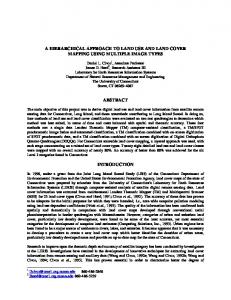
5. USING DSHP TO LEARN AN MDP 45000
MaxQ Rmax DSHP
40000
Number of Timesteps Until Optimal Behavior
Given a solution to the planning problem of Section 4, the learning algorithm is simple: Use experience to generate M ′ , then plan. If DSHP outputs a hierarchical-optimal policy we’re done. Otherwise, run the policy until an “unknown” (s, a) is found and repeat. It’s clear that the learning algorithm, which we call the Deterministic Sample-Based Hierarchical Learner (DSHL) will have sample complexity bounded by O(T ·U (M )), with U (M ) being the number of “unknown” state-actions that can be found, until the model M ′ is identical to M . For a flat and deterministic MDP M , U (M ) = |S| · |A|. In factored representations, U (M ) is often much smaller. By separating the hierarchy from the underlying representation, DSHL reaps the benefits of both forms of abstraction simultaneously.
35000 30000 25000 20000 15000 10000 5000 0 4
6
8
6. EMPIRICAL RESULTS We tested MaxQ, Factored Rmax and DSHL in the bitflip and the taxi domain ((Dietterich 2000c)). The results show that, as expected, Rmax has poor computational complexity and MaxQ has poor sample complexity. DSHL achieves both low computational and sample complexity.
10
12
14
16
18
20
22
Domain Size (Bits)
Figure 1: Number of steps per problem size until algorithm reaches optimal policy for the given start states. Rmax can only solve problems upto size 10, given the amount of time allocated.
6.1 Bitflip domain
1000
Computational time (milliseconds on logscale)
Our testing methodology was to evaluate the agent’s learned policy after each episode on a number of example states of the environment. The evaluation states were picked to follow a standard structure based on the number of bits n: all 1s (11..11), single 1 in the center (0..010..0), first half 1s (1..10..0), second half 1s (0..01..1), by quarters (1.10.01.10.0) and alternating 1s (101010...). Once an optimal policy is found, the trial stops and we record the cost (number of action choices) and computer time for the trial. Each experiment is repeated for 20 trials and all the results are averaged. We tested each algorithm on bitflip(n), where we allowed n to increase until one of two termination conditions were satisfied: when a value of n is reached for which the algorithm took longer than thirty minutes on a single trial, or when the number of action choices reached thirty thousand. Each algorithm has a number of parameters. For Factored Rmax, the main parameter is the Rmax constant κ. As we are dealing with a deterministic domain, this parameter was set to 1. For MaxQ, one must specify the value of ǫ for exploration and its decay rate. We did a search of these parameters (from 0.1 to 0.3, on 0.05 increments) and chose the setting that gave the best performance for each problem size. DSHL requires no parameter tuning. As we can see from the Figure 1, the sample complexity of both Factored Rmax and DSHL grows linearly in the number of factors of the domain, whereas the sample complexity of MaxQ grows exponentially. On the other hand, the computational cost for Factored Rmax grows exponentially (Figure 2), while both MaxQ and DSHL show polynomial growth rates. So, DSHL is the only algorithm to show polynomial growth rates in both sample and computational complexities, as predicted by our analyses.
MaxQ Rmax DSHP
100
10
1
0.1 4
6
8
10
12
14
16
18
20
22
Domain Size (Bits)
Figure 2: Computational time per step, per problem size. Plotted on a log scale, due to huge disparity between algorithms.
6.2 Taxi domain We used a similar testing methodology for the taxi domain described by Dietterich (2000c). We used the standard problem (no fuel, no fickle passenger) on a 5x5 grid. We used the same hierarchical structure and the same kind of abstractions used by MaxQ. The size of the problem in this case is fixed, so we only expose the good performance of DSHL in the two types of complexities. As in the previous problem, we evaluate the agent’s learned policy after each episode on a set of six starting combinations of . The start states used were: {(2, 2), Y, R}, {(2, 2), Y, G}, {(2, 2), Y, B}, {(2, 2), R, B}, {(0, 4), Y, R}, {(0, 3), B, G}. The results are shown in the following table: MaxQ Factored Rmax DSHL
Number of steps 6298 1839 319
Time per step 9.570ms 97.780ms 16.876ms
As can be seen, DSHL significantly improves the sample complexity of both MaxQ and Factored Rmax by combining models, factored state spaces and a hierarchal structure, while attaining low computational complexity comparable to that of MaxQ.
7. CONCLUSION We have designed a novel algorithm that combines factored representations, model-based learning, and hierarchies to provide a formal guarantee on learning time in many large deterministic reinforcement-learning domains. Empirical results indicate that, for a simple extensible class of MDPs, existing algorithms fail to provide either efficient sample complexity or efficient computational complexity. The results demonstrate, on the other hand, how the theoretical assurances of our hybrid algorithm translate to practical advantages.
8. REFERENCES [Boutilier et al., 1999] Craig Boutilier, Thomas Dean, and Steve Hanks. Decision-theoretic planning: Structural assumptions and computational leverage. Journal of Artificial Intelligence Research, 11:1–94, 1999. [Brafman and Tennenholtz, 2002] Ronen I. Brafman and Moshe Tennenholtz. R-MAX—a general polynomial time algorithm for near-optimal reinforcement learning. Journal of Machine Learning Research, 3:213–231, 2002. [Dietterich, 2000a] Thomas G. Dietterich. Hierarchical reinforcement learning with the MAXQ value function decomposition. Journal of Artificial Intelligence Research, 13:227–303, 2000. [Dietterich, 2000b] Thomas G. Dietterich. An overview of MAXQ hierarchical reinforcement learning. In Proceedings of the Symposium on Abstraction, Reformulation and Approximation SARA 2000, pages 26–44, 2000. [Dietterich, 2000c] Thomas G. Dietterich. State abstraction in MAXQ hierarchical reinforcement learning. In Advances in Neural Information Processing Systems 12, pages 994–1000, 2000. [Guestrin et al., 2002] Carlos Guestrin, Relu Patrascu, and Dale Schuurmans. Algorithm-directed exploration for
model-based reinforcement learning in factored MDPs. In Proceedings of the International Conference on Machine Learning, pages 235–242, 2002. [Hengst, 2002] B. Hengst. Discovering hierarchy in reinforcement learning with HEXQ. In Maching Learning: Proceedings of the Nineteenth International Conference on Machine Learning, pages 243–250. Morgan Kaufmann, 2002. [Kaelbling, 1993] Leslie Pack Kaelbling. Hierarchical learning in stochastic domains: Preliminary results. In Proceedings of the Tenth International Conference on Machine Learning, Amherst, MA, 1993. Morgan Kaufmann. [Kakade, 2003] Sham M. Kakade. On the Sample Complexity of Reinforcement Learning. PhD thesis, Gatsby Computational Neuroscience Unit, University College London, 2003. [Kearns and Koller, 1999] Michael J. Kearns and Daphne Koller. Efficient reinforcement learning in factored MDPs. In Proceedings of the 16th International Joint Conference on Artificial Intelligence (IJCAI), pages 740–747, 1999. [Kearns and Singh, 2002] Michael J. Kearns and Satinder P. Singh. Near-optimal reinforcement learning in polynomial time. Machine Learning, 49(2–3):209–232, 2002. [Koller and Parr, 2000] Daphne Koller and Ronald Parr. Policy iteration for factored MDPs. In Uncertainty in Artificial Intelligence, Proceedings of the Sixteenth Conference (UAI 2000), pages 326–334, 2000. [Moore and Atkeson, 1993] Andrew W. Moore and Christopher G. Atkeson. Prioritized sweeping: Reinforcement learning with less data and less real time. Machine Learning, 13:103–130, 1993. [Sutton and Barto, 1998] Richard S. Sutton and Andrew G. Barto. Reinforcement Learning: An Introduction. The MIT Press, 1998. [Sutton, 1990] Richard S. Sutton. Integrated architectures for learning, planning, and reacting based on approximating dynamic programming. In Proceedings of the Seventh International Conference on Machine Learning, pages 216–224, Austin, TX, 1990. Morgan Kaufmann. [Watkins and Dayan, 1992] Christopher J. C. H. Watkins and Peter Dayan. Q-learning. Machine Learning, 8(3):279–292, 1992.