System of systems engineering, which faces this problem on a large scale, cries out for a unifying ... simply because the opportunities for error grow with the.
A Unifying Framework for Systems Modeling, Control Systems Design, and System Operation Daniel L. Dvorak, Mark B. Indictor, Michel D. Ingham, Robert D. Rasmussen, Margaret V. Stringfellow Systems & Software Division Jet Propulsion Laboratory California Institute of Technology Pasadena, CA, USA {daniel.l.dvorak, mark.b.indictor, michel.d.ingham, robert.d.rasmussen, margaret.v.stringfellow}@jpl.nasa.gov Abstract – Current engineering practice in the analysis and design of large-scale multi-disciplinary control systems is typified by some form of decomposition— whether functional or physical or discipline-based—that enables multiple teams to work in parallel and in relative isolation. Too often, the resulting system after integration is an awkward marriage of different control and data mechanisms with poor end-to-end accountability. System of systems engineering, which faces this problem on a large scale, cries out for a unifying framework to guide analysis, design, and operation. This paper describes such a framework based on a state-, model-, and goal-based architecture for semi-autonomous control systems that guides analysis and modeling, shapes control system software design, and directly specifies operational intent. This paper illustrates the key concepts in the context of a large-scale, concurrent, globally distributed system of systems: NASA’s proposed Array-based Deep Space Network. Keywords: Systems modeling, control software design, human/machine systems.
1
architecture,
Introduction
The size and complexity of many systems being built for government, industry, and the military have reached a threshold where customary methods of analysis, design, implementation, and operation are no longer sufficiently reliable. Many of these large systems are properly described as “systems of systems” in that they are composed of many systems—often built by multiple suppliers—that must operate in a coordinated manner. The challenge of coordinated control almost always falls to software. Unfortunately, there is a fundamental gap between the requirements on software, as specified by systems engineers, and the implementation of those requirements by software engineers. Software engineers must perform the translation of requirements into software design and into code, trying to capture the systems engineer’s understanding of system behavior, which is not always explicitly specified. This gap can lead to serious
flaws in the implemented system, some of which may manifest at the most inopportune times. The twin problems of errors of omission and errors of interpretation are exacerbated in a system of systems simply because the opportunities for error grow with the number of system-to-system interactions that must be specified by systems engineers. They also grow with the number of different ‘mindsets’ about control mechanisms that different teams bring to the table, often based on reusable or legacy software. Another challenge in the validation of any complex software system is that much of what transpires in software design and development is opaque to systems engineers. It is nigh impossible for a systems engineer to obtain a description of the software design that is simultaneously faithful to the software as built and expressed in terms directly related to the requirements. Too often, software designs presented at reviews are box-and-line diagrams that amount to an appealing fiction; they present an idealized design that fails to reveal all of the interactions built into the software. This paper describes a systems engineering methodology called State Analysis [2], intended for application to autonomous and semi-autonomous control systems. State Analysis asserts four basic principles:
Control subsumes all aspects of system operation. It can be understood and exercised intelligently only through models of the system under control, so a clear distinction must be made between the control system and the system under control.
Models of the system under control must be explicitly identified and used in a way that assures consensus among systems engineers.
Understanding state is fundamental to successful modeling. Everything we need to know and everything we need to do can be expressed in terms of the state of the system under control.
As complexity grows, the line between specifying behavior and designing behavior is blurring. The software design must reflect the systems engineer’s understanding, so the manner in which models inform software design and operation should be direct, requiring minimal translation.
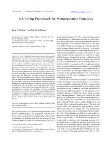
As Figure 1 depicts, this methodology addresses the trinity of system analysis, software design, and operational control. These three aspects of a system must be mutually consistent to achieve a reliable and understandable end product. The unifying principles for these three aspects form the foundation of a state- and model-based control architecture for systems of systems. This paper illustrates the application of State Analysis and the state- and modelbased control architecture in the context of globally distributed, concurrent control system. System operations scenario
guides Analysis of system under control
produces Physics model of system under control
informs
informs Control system software
operates
Goal elaborations for operations
Figure 1. State Analysis provides a unified approach to system analysis, control system software design, and system operation.
2
The Deep Space Array Network
This paper examines NASA’s proposed Deep Space Array Network (DSAN) as a case study in system of systems engineering. DSAN is designed to be the nextgeneration network of Earth-based antennas that provide communication services to NASA’s deep space missions of exploration [4]. According to current plans, the network will contain 1200 12-meter receive antennas, divided equally among three longitudes (“regions”) in order to maintain tracking as the Earth rotates. As the name implies, DSAN employs sophisticated digital signal processing to combine signals from an array of antennas in order to achieve the effective aperture of a much larger antenna. With 400 antennas at each of the three regions, numerous target spacecraft can be tracked concurrently by allocating
groups of antennas to each target and routing their signals appropriately through the signal processing system. DSAN is a system of systems in that it is composed of multiple complex systems, is geographically distributed, and must be coordinated and controlled as a single system. Kotov’s definition [1] is particularly apt: “Systems of systems are large scale concurrent and distributed systems that are comprised of complex systems.” DSAN is comprised of several complex systems including: the receive array; transmit array; large transmit/receive array; telemetry, ranging, and command processing; very long baseline interferometry processing; frequency and timing; and monitor & control. This paper focuses on monitoring & control for the receive array. There are three levels of automated monitoring & control within DSAN. At the lowest level, closest to the hardware, hard real-time control loops read sensors and command actuators to do things such as pointing the antennas, configuring the signal flow and signal processing, and constantly monitoring for anomalies. At the next level up—the regional level—the job is to allocate and manage all the resources, including the 400 antennas of the receive array at each region, in the service of customer requests for spacecraft tracking. The regional level must respond to faults in real time, such as quickly replacing a failed antenna in an active array. The final level of monitoring & control is at DSAN Central. This top level assigns work to each of the three regions, based in part on what regions have a spacecraft’s signal “in view” at the time its signal is reaching Earth. As with regional control, central control must react in real time to anomalies reported by each region. For example, DSAN Central could direct the Australian region to start tracking a spacecraft earlier than expected if a failure occurs in the California region.
3
State Analysis
State Analysis is a systems engineering process for the problem domain of autonomous and semi-autonomous control systems. It is a comprehensive process in that it addresses analysis of the system to be controlled, design of the control system, and operation of the control system. Compared to more conventional systems engineering processes, it demands more up-front analysis and it represents its results in a more structured form. Its main benefit is more reliable systems due to fewer errors of omission, fewer errors of translation into software, and more easily understood operational controls. It also enables more accurate cost estimation because there is a much more direct mapping from analysis artifacts to units of work. A detailed presentation of the State Analysis methodology is found in reference [2]. In this paper, we introduce the fundamental architectural concepts of the approach, and describe its application to the DSAN system of systems.
3.2
Control System Planning & Execution
Knowledge Goals
State Functions State Estimation
Control Goals State Knowledge
State Values
Models
Measurements & Commands
State Control Commands
Hardware Adapter
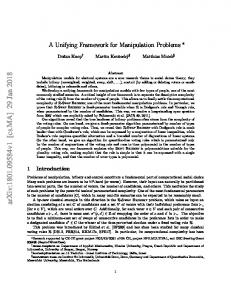
System Under Control Figure 2. Architecturally, State Analysis emphasizes a clear distinction between the control system and the system under control, with explicit representation off State variables and behavioral models.
3.1
Architectural Concepts
To understand State Analysis, it is important to understand a few architectural features that shape it, as depicted in Figure 2. First, there is a clear distinction between the control system and the system under control because control can only be understood and exercised intelligently through models of the system under control. Second, state variables of the system under control are explicit since it is the values of those state variables that the control system is designed to control. Third, models of how the system under control behaves are documented explicitly because they are needed by the control system for execution (estimating and controlling state) and higherlevel planning (e.g. resource management). Fourth, state estimation is separate from state control because separation promotes objective assessment of system state and ensures consistent use of state across the control system. Fifth, hardware adapters provide the sole interface between the control system and the system under control, with all interactions in the form of commands to and measurements from the system under control. Sixth, the architecture emphasizes goal-directed closed-loop operation because goals, as constraints on the values of state variables over time intervals, directly express operational intent. Finally, the architecture provides a straightforward mapping into software because the aforementioned architectural concepts (state variables, models, estimators, controller, measurements, commands, goals) are represented directly in software.
Modeling of the System Under Control
As a systems engineering process, State Analysis is a gradual discovery process that is incremental in nature, and each increment can expand the analysis in terms of scope or detail, or both. The process is all about understanding and modeling the system under control since the control system needs such models. The first steps of the process are: (1) identify the state variables of the system under control that must be monitored and/or controlled; (2) identify the direct effects of one state variable on another (state-to-state effects); (3) identify the measurements that provide evidence about the values of state variables (stateto-measurement effects); and (4) identify the commands that affect the state variables (command-to-state effects). All of these state variables, measurements, commands, and influences are captured in a “physics model”, so named because it captures the physics of the system under control. Figure 3 provides an overview of a portion of the physics model centered around a state variable for the operational mode and health of an antenna mechanical system. The incoming arrows to that state variable show that its value is affected by facility power (another state variable) and mechanical mode commands. The outgoing arrows show that the value of this state variable affects the received signal (another state variable) as well as four measurements (antenna pointing, motor current, mechanical operating mode, and antenna mechanical power). Figure 4 shows a statechart (a behavioral model) that expresses behaviors of the system under control related to an antenna’s operating mode and health. Specifically, it shows how the power state and mode commands affect the antenna operational mode and how different measurements provide evidence about the value of that state variable. Cmd: Mech. OpMode
Antenna Power
Antenna Mechanical OpMode & Health Msmt: Antenna Pointing
Msmt: Antenna Mech. Power Msmt: Motor Current
Legend :
Msmt: Mech. OpMode
= state variable = measurement = command
Figure 3. This view of the physics model shows what affects what among the state variables, commands, and measurements of the antenna mechanical system.
Healthy high motor current
Offline & not ready
motor repaired
Cmd: go offline
Unhealthy
Offline & ready Cmd: go online
Shutdown
Tracking Off-pnt msmt
Msmt: “repaired”
Power off
Power off
On point On-pnt msmt
Begin tracking
End of profile or go-idle
Off point
Stowing
Power off Stow
Power on Stowed or go-idle
Idle
Figure 4. Statechart model for antenna mechanical system. Although this example employs a statechart, in principle a model can be described in a variety of ways including equations, tables, pseudo-code, and text. The key requirement is that the model must unambiguously specify behavior, i.e. how the system under control works. As is always true in systems engineering, the level of detail that a system engineer decides to capture in a physics model should be driven by need. The model should make explicit all the effects and behaviors of the system under control that must be known to properly control it. Effects that are present but considered insignificant should be so noted so that such assumptions are recorded and reviewable. Importantly, the graphical representation of a physics model shold be easy to review with domain experts and other systems engineers. Graphical representations, as shown in Figures 3 and 4, are particularly appropriate.
Cmd: Mech. OpMode
Antenna Power
Antenna Mechanical OpMode & Health Msmt: Antenna Pointing Msmt: Mech. OpMode
Control System Software Design
An important aspect of the architectural concepts outlined in section 3.1 is that the same concepts of states and models that shape the State Analysis process also shape the reference architecture for the software. The right-hand side of Figure 5 shows a UML collaboration diagram that mirrors the architectural concepts depicted in Figure 2. Figure 5 presents a control loop pattern for the antenna mechanical op mode and health. In this pattern an estimator repeatedly reads measurements and commands from the system under control, interprets them with respect to measurement models and command models (part of the physics model), and updates the current estimated state. A controller repeatedly compares estimated state to desired state (represented in a control goal), and issues commands, as appropriate, to the system under control. The decision of what command to issue, if any, depends on the command Knowledge goal
Control goal
State Variable: Ant. Mech. OpMode & Health
updateState
Msmt: Antenna Mech. Power Msmt: Motor Current
3.3
Estimator: Ant. Mech. OpMode & Health
getState Controller: Ant. Mech. OpMode & Health
readMeasurements sendCommand readCommands Hardware Adapter: Antenna Mechanical System
Figure 5. The physics model (shown on the left) directly informs the software design (shown on the right). The physics model elements (state variables, measurements, and commands) and the models behind them (state, measurement, and command effects models) all map into the software design.
effects model (also part of the physics model). As Figure 5 shows, there is a direct mapping between elements in the physics model and elements in the software design. For every state variable in the physics model there is a state variable component in the collaboration diagram. For every state variable there is exactly one estimator, and its job is to interpret all evidence about the state (the value) of the state variable. The specific kinds of evidence are all identified in the physics model. For example, every measurement in the physics model that is affected by the physical state known as Antenna Mechanical OpMode & Health becomes input to its estimator component. Similarly, commands and physical states that affect the state of the state variable also become inputs to the estimator. Although not shown in this example, an estimator may also use the value of an affected state variables as evidence. In all cases, the estimator uses information in the physics model (state-to-state effects, state-to-measurement effects, and command-to-state effects) to properly interpret all the evidence. A similar mapping exists for controllers. For every controllable state variable in the physics model there is exactly one controller, and its job is to issue commands, as needed, to achieve a desired state, as expressed in a control goal. A goal is defined as a constraint on the values of a state variable over a time interval, so a controller’s job is to try to keep the constraint satisfied by influencing the physical state of the system under control. In general, a controller may issue more than one kind of command to more than one kind of subsystem, but only if those commands affect the controlled state variable, as identified in the physics model. Estimators take into account the predict effects of an issued command by getting a copy of the issued command, plus its timestamp, from the system under control. The key point here is that the direct mapping of analysis artifacts to software design eliminates many Parent goal
Goal
opportunities for error. Compared to “shall” statements, these analysis artifacts are highly structured and unambiguous. Using framework software elements that mirror the analysis artifacts, software engineers make far fewer errors of interpretation, and the system as built bears a direct resemblance to the analysis artifacts.
3.4
The preceding section showed how a portion of a physics model informed the software design for a single control loop. Each individual control loop is controlled by a pair of goals: a control goal for the controller and a knowledge goal for the estimator. In simple terms, a control goal specifies a desired state (or desired state history) and a knowledge goal specifies a required quality of knowledge about estimated states. For example, in the control loop for antenna mechanical operating mode and health, a control goal might specify that the antenna is healthy and that the antenna system is tracking and onpoint. A corresponding knowledge goal might specify that antenna operating mode and health is known with high confidence. Goals provide an excellent basis for operations because they directly specify intent (i.e. “what” rather than “how”) and because they are checkable during operation (a goal is said to “fail” if its constraint is violated). In any real system there are many state variables, often numbering in the thousands, and so there is a need to coordinate hundreds or thousands of control loops. In our architecture such coordination is accomplished via a goal network. A goal network typically begins with the specification of a few high-level goals and then expands through a process of goal elaboration and scheduling. Goal elaboration is the process of specifying the child goals (subgoals) needed to achieve a particular parent goal. For example, for an antenna mechanical system to be tracking and on-point (a parent goal), it must have power and its operational mode must be known (two child goals).
Time-point
Child goals (subgoals) from first level elaboration
Ant Mech OpMode & Health: Healthy, Tracking & On-point
Antenna Power: Is Known and Powered Ant Mech OpMode & Health: Transition to Healthy, Tracking & On-point
Grandchild goals from 2nd level elaboration
Goal Elaborations for Operations
Ant Mech OpMode & Health: Is known
Antenna Power: Transition to Powered Ant Mech OpMode & Health: Is Known
Figure 6. Goal elaborations are the building blocks for operation of the control system. A parent goal specifies a constraint on state to be satisfied during a time interval, denoted by starting and ending time-points. The elaboration specifies required subgoals, as directly informed by state-to-state effects in the physics model.
Interestingly, such goal elaborations are informed by the same physics model described previously. These elaborations are constructed by applying four simple rules to the model: (1) a goal on a state may elaborate to a control subgoal on an affecting state; (2) a control goal on a state elaborates to a knowledge goal on the same state; (3) a knowledge goal on a state may elaborate to knowledge goals on its affecting and affected states; and (4) a “maintenance” goal on a state may elaborate to a “transition” goal on the same state, with an ending timepoint coincident with the starting time-point of the maintenance goal. Figure 6 depicts the results of applying these rules to a parent goal that the antenna mechanical op mode and health state variable be in the state of health, tracking, and on-point. It should be noted that alternative ways of accomplishing a goal are specified via multiple alternative goal elaborations, called tactics. Thus, should any of the supporting goals in an elaboration fail, it becomes possible to re-elaborate with an alternate tactic to accomplish the same objective. Context-specific elaboration can be enabled by conditioning alternative elaboration tactics on different state constraints. There is more to the story of goal-based operations that is beyond the scope of this paper, including additional detail on the elaboration process (see [2]) and a thorough explanation of scheduling and executing goal networks (see [2,5]). The basic idea is that one or a few high-level goals are specified by operators and then a process of goal elaboration and scheduling produce a schedule of operations. In the case of the Deep Space Array Network, a high-level goal in the form of a mission service request would start such a process. Such a goal might specify that the mission customer wants to receive at least 98% of the data frames from a downlink pass from spacecraft x. The elaboration of that goal would, among other things, use knowledge of the spacecraft trajectory, modulation format, data rate, and radiated power to determine how many antennas need to be arrayed together to receive the data with the level of certainty specified by the customer.
4
Conclusions
This paper has shown how the architectural concepts of state variables, models, and goals provide a unified view of control that shapes the trinity of system analysis, software design, and operational control. Analysis is always about the system under control, not the control system, and it begins with a discovery process for state variables, commands, and measurements, plus the models of behavior that relate them. The software design is always about the control system, whose job is to monitor and control specific state variables in the system under control. To do this it depends on knowledge of how the system under control works — exactly the same knowledge of behavior captured in the models. Estimators, controllers,
and planning & execution in the software design all use the models. Finally, operational control via goal networks is designed in accord with the physics model, for both nominal operations and fault responses. Specifically, goal elaborations and their alternate tactics are employed directly during system operation to effect coordinated control of the whole system. The important message in this paper is that complex systems can be built more reliably if a unified approach is followed. By adopting the State Analysis approach, elements of the physics model map directly onto software design, and state-to-state effects directly shape the goal elaborations. The system as built is no longer opaque to systems engineers because it now represents the results of their analysis in a direct, inspectable way. As is the case in the Deep Space Array Network, it’s not necessary that all of the software-based control in a system of systems be designed and built in the manner described here. Systems or subsystems implemented using a different design may be viewed as part of the system under control and their “black box” behaviors would therefore be modeled during analysis. For more information about State Analysis and its underlying architecture see [2,3,5].
References [1] V. Kotov, “System of systems as communicating structures,” Hewlett Packard Computer Systems Laboratory Paper HPL-97-124, pp. 1-15, 1997. [2] M.D. Ingham, R.D. Rasmusen, M.B. Bennett, and A.C. Moncada, “Engineering complex embedded systems with state analysis and the mission data system,” American Institute of Aeronautics and Astronautics Conference on Intelligent Systems, Chicago, Sep. 2004. [3] D. Dvorak, R. Rasmussen, G. Reeves, and A. Sacks, “Software architecture themes in JPL’s mission data system,” IEEE Aerospace Conference, Big Sky, March 2000. [4] D.S. Bagri, J.I. Statman, and M.S. Gatti, “Operations Concept for Array-based Deep Space Network,” IEEE Aerospace Conference, Big Sky, March 2005. [5] A. Barrett, R. Knight, R. Morris, and R. Rasmussen, “Mission Planning and Execution Within the Mission Data System,” Proceedings of the International Workshop on Planning and Scheduling for Space, Darmstadt, June 2004.