Hybrid Automata as a Unifying Framework for Modeling ... - CiteSeerX

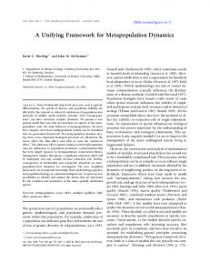
Hybrid Automata as a Unifying Framework for Modeling Excitable Cells P. Ye, E. Entcheva, S.A. Smolka, M.R. True and R. Grosu Abstract— We propose Hybrid Automata (HA) as a unifying framework for computational models of excitable cells. HA, which combine discrete transition graphs with continuous dynamics, can be naturally used to obtain a piecewise, possibly linear, approximation of a nonlinear excitable-cell model. We first show how HA can be used to efficiently capture the actionpotential morphology—as well as reproduce typical excitablecell characteristics such as refractoriness and restitution— of the dynamic Luo-Rudy model of a guinea-pig ventricular myocyte. We then recast two well-known computational models, Biktashev’s and Fenton-Karma, as HA without any loss of expressiveness. Given that HA possess an intuitive graphical representation and are supported by a rich mathematical theory and numerous analysis tools, we argue that they are well positioned as a computational model for biological processes.

I. I NTRODUCTION In this paper, investigate the use of Hybrid Automata (HA) as a formal modeling language for excitable cells in general, and cardiac cells in particular. HA combine discrete transition graphs with continuous dynamics. Traditionally, they were used as models for a variety of embedded systems, including automated highway systems, air traffic management, embedded automotive controllers, robotics and realtime circuits. More recently, they have been used to model molecular and cellular systems [1]. The formal definition of an HA is given as follows. A hybrid automaton is an extended finite automaton where each state is endowed with a continuous dynamics [2]. Consequently, an HA consists of: (i) A finite set X of realvalued variables x1 , . . ., xn ; their dotted form x˙i ∈X˙ represents first derivatives and their primed form xi ∈X  represents values at the conclusion of discrete steps. (ii) A finite control graph (V, E), where vertices in V are called modes and edges in E are called switches. (iii) Vertex-labeling functions init, inv and flow assigned to each mode v∈V . Initial condition init(v) and invariant inv(v) are predicates with free variables from X. Flow flow(v) is a predicate with free variables from X∪X˙ representing a set of ordinary differential (in)equations. (iv) An edge-labeling function jump assigned to each switch e∈E. Jump jump(e) is a predicate with free variables from X∪X  and is usually divided into a guard and an assignment action. (v) A finite set Σ of events, and an edge-labeling function event that assigns to each switch an event. Research supported in part by NSF Grant CCF05-23863 and NSF CAREER Grant CCR01-33583 E. Entcheva, R. Grosu and S.A. Smolka are IEEE members P. Ye, R. Grosu, S.A. Smolka and M.R. True are from Computer Science department, Stony Brook University, Stony Brook, NY 11790, USA E. Entcheva is with the Department of Biomedical Engineering, Stony Brook University, Stony Brook, NY 11794, USA

Mode OFF

x = 20

Fig. 1.

x˙ = −0.1x {x ≥ 18}

[x > 21]

Mode ON

x˙ = 5 − 0.1x [x < 19]

{x ≤ 22}

A thermostat system modeled as an HA

An HA has a natural graphical representation as a state transition diagram, with control modes as the states and control switches as the transitions. Flows and invariants (predicates within curly braces) appear within control modes, while jump conditions (in square brackets) and actions appear near the control switches. Continuous variables are written in lower case (x, v, vx , etc). A simple example of an HA for a thermostat system is illustrated in Fig. 1. Initially the system is in mode OFF and the initial value for variable x, which represents the current temperature, is 20°C. In mode OFF, the heater is off and the temperature drops until it falls below 19°C. At this point, the switch from mode OFF to ON occurs. In mode ON, the heater is on and the temperature rises until it is above 21°C. At this point, the switch from mode ON to OFF occurs. The rest of the paper is organized as follows. Section II surveys recent applications of HA to different biological systems. Section III presents our Luo-Rudy-inspired HA model for the guinea-pig cardiac myocyte. Section IV describes a systematic method for transforming any dynamic system defined in terms of Heaviside functions into an equivalent HA. Section V shows how this technique can be used to rewrite two popular simplified ionic models into the HA framework: Biktashev’s simplified model for wave propagation [3] and the Fenton-Karma model [4]. The diversity of these models illustrates the generality of the HA approach. Section VI contains our concluding remarks and directions for future work. II. H YBRID AUTOMATA FOR B IOLOGICAL S YSTEMS Hybrid Automata start finding applications as a formalmodeling tool in both intracellular and intercellular biological applications. Many biological systems are “hybrid” in nature: concentrations of different biological species may vary continuously, yet discrete transitions between distinct states are also possible. Excitable cells are a good example of such hybrid systems - transmembrane ion fluxes and transmembrane voltage may vary continuously but transition from resting to excited state is generally considered all-or-nothing discrete response. Furthermore, networks of biological entities (genes, molecules, cells) tend to exhibit properties such as concurrency and communication, for which automatabased formalisms are well developed [5].

Currently, the preferred modeling approach for biological systems requires solving large sets of coupled nonlinear differential equations. In contrast, HA-based models provide piece-wise linear approximation, which leads to simplicity, possibility for easy scale-up, large scale simulations and formal analysis. The construction of HA models can be approached in a couple of ways. For example, abstraction can be applied to both the modes and the changes in a dynamic system. In [1], a protein-regulatory network was investigated. Each of two interacting proteins was associated with two modes: active and non-active. In each mode, a linear dynamic function was used to describe the concentration change of that protein. HA models constructed using abstraction tend to be of low complexity as well as low precision, but are suitable for large-scale simulation and further analysis. Alternatively, a system of coupled nonlinear ordinary differential equations (ODEs) describing processes with disparate time scales can be simplified and transformed into an HA model. This usually entails substitution of the fasttransitioning continuous functions with a Heaviside function, and/or assumptions that certain variables remain constant within a mode if they do not vary extensively [3]. Furthermore, if a formal mathematical model is not available, a completely empirically-rooted HA derivation can be applied using experimental data [6]. Each time step can be associated with a mode. If the data set is large, the resulting system would be large as well. However, simplification techniques based on HA can be used to reduce the overall complexity, making this method feasible for real applications. Once a valid HA model has been developed, it can be used to explore the parameter space and to apply formal analysis of the biological systems under investigation. Of great interest for dynamic systems are: stability and reachability analysis. The former has been applied to HA models for a single entity [7] as wells as for a network of interacting elements [8]. Reachability analysis is generally an NPcomplete or undecidable computational problem. However, a number of approximation techniques have been developed recently for the reachability analysis of biological systems represented by HA ([9], [10], etc.). III. HA M ODELS FOR C ARDIAC C ELLS In this section, we present our HA model of a guinea-pig ventricular myocyte. We use the popular LRd model [11], [12] for validation of cell behavior. (For the details of our HA model, please refer to [13].) A. Background At the cellular level, an electrical signal is a change in the potential across the cell membrane, caused by the flow of ions between the inside and outside of the cell. The electrical signal at the cellular level for each excitation event is known as an action potential (AP). The time period during which a cell stays at its excited state (when the voltage is relatively high) is called the action-potential duration (APD).

Early Repolarization Plateau

Upstroke

Final Repolarization

Stimulated

Fig. 2.

Resting

AP phases and corresponding HA modes

An important property for cardiac cells is that a longer recovery time is followed by a longer APD. The physiological explanation is rooted in the ion-channel kinetics as a limiting factor in a cell’s frequency response. This property is called AP restitution. B. The HA Model We present a four-state HA model matching the LRd cardiac-cell behavior. Our interest lies in the correct capture of AP morphology and the key properties of excitable cells: refractoriness and restitution. The detailed behavior of each ion channel is not our target. To this end, the equations in each control mode mainly serve as curve-fitting formulae and may not reflect the physical quantities of different biological entities except for the membrane potential v. The intuition behind the HA model is that we first associate a control mode with each major AP phase: resting and final repolarization (FR), stimulated, upstroke, and plateau and early repolarization (ER). Initially, the cell is in resting and FR mode. When (externally) stimulated with the event VS , it enters mode stimulated and updates its voltage according to the stimulus current. Upon termination of the stimulation, via event V S , with a sub-threshold voltage, the cell returns to resting mode without firing an AP. If the stimulus is supra-threshold, i.e., v ≥ VT holds, the excited cell will generate an AP by progressing to mode upstroke. The recovery course of the cell follows transitions to mode plateau and ER and then to resting and FR mode. It is important to note that the HA model does not impose a rigid timing scheme, but instead possesses inherent voltage dependence, i.e. the jump conditions monitor transmembrane potential V. This approach allows for AP adaptation (response to various pacing frequencies). The transition relation of HA model also reflects the refractory period of excitable cells. Only during mode resting and FR, the cell can respond to external stimuli, thus this period is defined as relative refractory period. In other modes, the cell will not be responsive, thus it is within absolute refractory period. The relation of control modes in the HA model with different AP phases is described in Fig. 2. The HA introduced so far has no memory. Hence it will produce the same AP every cycle. To accommodate adaptability to pacing frequency, we introduce a memory unit, vn , which remembers the current voltage every time a new stimulus is arriving. The value of vn will control the AP morphology of the current cycle, thus make APD adaptive

q0 : Resting & FR v˙ x = αx0 vx , v˙ y = αy0 vy , v˙ z = αz0 vz v = vx − vy + vz

[Vs ] vn = v [v < VT ∧ V¯s ]

{v < VR }

q1 : Stimulated

{v < VT } [v ≥ VT ]

v˙ z = αz3 vz , v = vx − vy + vz {v < VO ∧ v > VR }

Fig. 3.

v˙ = f (0, y) {x < 0}

v = vx − vy + vz

[v ≤ VR ]

Fig. 4.

q2 : Upstroke v˙ x = αx2 vx, v˙ y = αy2 vy , v˙ z = αz2 vz

q3 : Plateau & ER v˙ x = αx3 vx f (θ), v˙ y = αy3 vy [v ≥ VO ]

v = vx − vy + vz

q0 E˙ = ∇(D∇E)

[E = 0]

[E = 0]

{E ≤ 0}

Hybrid automaton for guinea pig cardiac myocyte.

Fig. 5.

to DI. Let θ = vn /VR , where the value of vn is the one in the current mode and VR serves as a threshold between cell’s absolute refractory period and relative refractory period. Only when the cell is in resting mode where the membrane potential v ≤ VR , the value of vn could be reset. Thus we have 0 < θ ≤ 1. Fig. 3 gives the HA model for LRd. Constant parameters in the flows are in lower-case Greek (αx0 , etc); constants in invariants and jump conditions (VT , etc), as well as events (VS√ ), are in upper case. We incorporate function f (θ ) = 1 + 13 6 θ (our choice of a 6th root function is inspired by the fact that the APD is not proportional to DI but a convex function of it) into mode Plateau and ER, which determines the length of the APD. The choice of the parameters here is to give the best match of both AP morphology and restitution as seen in the LRd model. C. Simulation Results In [13], we present simulations results for our HA model for both a single AP and for the restitution property. A comparison with the LRd model reveals that, with much less complexity, our HA model accurately captures the AP morphology and adaptation to pacing frequency. IV. F ROM H EAVISIDE TO H YBRID In recent attempts to construct simplified models of cardiac excitation, the Heaviside function has been used to achieve piecewise control and change of modes. Such discrete transitions are an integral part of the HA formalism. Below we present a systematic way to transform any dynamic system defined using Heaviside functions into an equivalent HA. The Heaviside function H(x) is a discontinuous function defined as follows:
0, x < 0; H(x) = (1) 1, x ≥ 0. Suppose the state equation in a mathematical model containing the Heaviside function is of the following form: (2)

Then (2) can be transformed into an HA with two control modes as shown in Fig. 4. It is obvious that the HA of Fig. 4 will behave exactly the same as the system in (2) (the switches are transient).

[x < 0]

Mode 1

v˙ = f (1, y) {x ≥ 0}

HA transformed from Heaviside function

h˙ = τ1 (1 − h)

{v < VO ∧ v > VT }

v˙ = f (H(x), y),
v = (x,
y)

[x ≥ 0]

Mode 0

v˙ x = ist , v˙ y = αy1 vy , v˙ z = αz1vz

q1 E˙ = ∇(D∇E) h˙ = τ1 (−h) {0 < E < 1}

[E = 1]

[E = 1]

q2 E˙ = ∇(D∇E) + h h˙ = τ1 (−h) {E ≥ 1}

Biktashev’s model in HA framework

In this way, all dynamic systems whose state equations are defined using Heaviside functions can be transformed into HA without any loss of information. V. P REVIOUS M ODELS V IEWED IN THE HA F RAMEWORK A. Biktashev’s Model The increasing complexity of modern models of excitable cells describing AP triggered a continuous effort to simplify these models. We take Biktashev’s simplified model as an example. (The justification and validation of his simplified model will not be discussed here.) After applying the approximation methods mentioned in Section II, Biktashev obtained the following simplified model: E˙ = ∇(D∇E) + H(E − 1)h

(3)

1 (4) h˙ = (H(−E) − h) τ where H is the Heaviside function, E is the transmembrane voltage, h is the probability density of sodium channel gate being open and τ is treated as a constant. E˙ and h˙ represent the time derivatives of the state variables E and h. The term ∇(D∇E) is the second order directional derivative on the 2-D space, which represents the diffusion factor when modeling the spatial propagation of cell excitations. The transformation process for Heaviside functions discussed in Section IV yields the HA of Fig. 5. The HA has three modes, the number of modes determined by the number of different values that make the input of the Heaviside function zero. Although Biktashev’s model and our HA model are both piecewise-linear approximations of LRd, only our HA model reproduces the correct AP morphology. B. The Fenton-Karma Model The Fenton-Karma 3-variable ionic model simplifies complicated ionic models by grouping different ion currents to achieve minimal ionic complexity. The ion currents in the model are fast inward current I f i , slow outward current Iso and slow inward current Isi . The corresponding 3-variable model contains dynamic functions for variable u (normalized membrane voltage), inactivation-reactivation gate variable v for I f i and gate variable w for Isi (the diffusion term is omitted here):

q0 :

q1 :

u˙ = −Jf i − Jso − Jsi + Jstimulus v˙ = (1 − v)/τv−1 w˙ = (1 − w)/τw− Jf i = 0 Jso = τu0 Jsi = − 2τwsi (1 + tanh(k(u − usi c )))

u˙ = −Jf i − Jso − Jsi + Jstimulus

{0 < u < uv }

[u = uv ] v˙ = (1 − w˙ = (1 − w)/τw− Jf i = 0 Jso = τu0 Jsi = − 2τwsi (1 + tanh(k(u − usi c ))) v)/τv−2

{uv ≤ u < uc}

[u = uc]

[u = uc] q2 :

q3 : u˙ = −Jf i − Jso − Jsi v˙ = (1 − v)/τv+ w˙ = (1 − w)/τw+

u˙ = −Jf i − Jso − Jsi + Jstimulus + stimulation v˙ = (1 − v)/τv

Jf i = − τvd (1 − u)(u − uc)

Jso =

Off

1 τr

Jsi = − 2τwsi (1 + tanh(k(u − usi c )))

{uc ≤ u}

Fig. 6.

w˙ = (1 − w)/τw+ Jf i = − τvd (1 − u)(u − uc) Jso = τ1r Jsi = − 2τwsi (1 + tanh(k(u − usi c ))) {uc ≤ u}

Fenton-Karma 3-variable ion-currents model in HA framework

u˙ = −J f i (u; v) − Jso (u) − Jsi (u; w)

(5)

v˙ = H(uc − u)(1 − v)/τv− (u) − H(u − uc )v/τv+

(6)

w˙ = H(uc − u)(1 − w)/τw− − H(u − uc )w/τw+

(7)

J f i (u; v) = − Jso (u) =

v H(u − uc )(1 − u)(u − uc ) τd

(8)

u 1 H(uc − u) + H(u − uc ) τo τr

(9)

w (1 + tanh[k(u − usic ]) 2τsi

(10)

Jsi (u; w) = −

where J f i (u; v), Jso (u) and Jsi (u; w) are the normalized versions of I f i (u; v), Iso (u) and Isi (u; w) respectively. uc and usic are the threshold potentials for activation of I f i and Isi . τv+ , τw− , τw+ , τd , τo , τr and τsi are time constants. τv− (u) is further defined by the Heaviside function:

τv− (u) = H(u − uv )τv−1 + H(uv − u)τv−2

(11)

where uv is the threshold potential, τv−1 and τv−2 are time constants. The HA for the Fenton-Karma model is depicted in Fig. 6. It was derived by taking into account the on-off status of an outside stimulus current Istimulus (omitted in the above equations), together with the definition of the Heaviside functions given above. The Fenton-Karma model has the flexibility to match AP morphology by correct selection of the parameters. However, the resultant simplified system is still highly nonlinear and difficult to treat analytically. VI. C ONCLUSIONS We proposed the use of Hybrid Automata as a unifying model for contemporary ionic-channel approximation techniques. Representing the complex response of excitable cells with piecewise-linear HA models permits fully analytical solutions in the different phases of the excitation cycle, therefore providing a framework for analytical analysis regardless

of the complexity of the system. Additionally, the piecewise linearization of the system and the simplified description increase computational efficiency to get numerical solutions (when analytical solution is impossible) without abstracting away essential system features. We have implemented the HA approximation for both neuron models and cardiac ion models and successfully captured spiral waves in 2-D simulations of cell arrays with markedly reduced simulation times [13]. Furthermore, we have shown how to recast two popular approximation models as HA. The graphic representation is easier to understand while still remaining a fully formal model. Future work includes the analytical analysis of stability based on the derived HA, and the mathematical exploration of arrhythmia-prone (unstable) modes. To further improve the efficiency of simulation, we are currently implementing additional optimization techniques for our HA models. All together they will make large-scale simulations of cardiac tissue possible. R EFERENCES [1] R. Ghosh and C.J. Tomlin, Lateral inhibition through Delta-Notch signaling: a piecewise affine hybrid model, Lecture Notes in Computer Science, vol 2034, 2001, pp 232-246. [2] T.A. Henzinger, “The theory of hybrid automata”,in Proceedings of the 11th IEEE Symposium on Logic in Computer Science, 1996, pp. 278-293. [3] V.N. Biktashev, A simplified model of propagation and dissipation of excitation fronts, Int. J. Bifurcation and Chaos, vol. 13, 2003, pp 3605-3620. [4] F. Fenton and A. Karma, Vortex dynamics in 3D continous myocardium with fiber rotation: filament instability and fibrillation,CHAOS, vol. 8, 1998, pp 20-47. [5] R. Milner, Communication and Concurrency, Prentice Hall, International Series in Computer Science, 1989. [6] M. Antoniotti and C. Piazza and A. Policriti and M. Simeoni and B. Mishra, Taming the complexity of biochemical models through bisimulation and collapsing: theory and practice. Theor. Comput. Sci, vol. 325, 2004, pp 45-67. [7] J.G. Dumas and A. Rondepierre, “Modeling the electrical activity of a neuron by a continuous and piecewise affine hybrid system”, Hybrid Systems: Computation and Control, 2003, pp 156-171. [8] C. Belta and J. Schug and T. Dang, “Stability and reachability analysis of a hybrid model of luminescence in the marine bacterium Vibrio fischeri”, In preceeding of 40th IEEE conference on Decision and Control, vol. 1, 2001, pp 869-874. [9] R. Alur and T. Dang and F. Ivancic, Reachability analysis of hybrid systems via predicate abstraction. In the preceeding of HSCC, 2002, pp 35-48. [10] R. Ghosh and C. J. Tomlin, Symbolic reachable set computation of piecewise affine hybrid automata and its application to biological modeling: Delta-Notch protein signaling, IEE Tansactions on Systems Biology, Vol. 1, 2004, pp 170-183. [11] C.H. Luo and Y. Rudy, A model of the ventricular cardiac action potential - depolarisation, repolarisation and their interaction, Circulation Research, vol. 68, 1991, pp 1501–1526. [12] C.H. Luo and Y. Rudy, A dynamic model of the cardiac ventricular action potential: I. Simulations of ionic currents and concentration changes, Circulation Research, vol. 74, 1994, pp 1071-1096. [13] P. Ye and E. Entcheva and R. Grosu and S.A. Smolka, “Efficient modeling of excitable cells using hybrid automata”, In Proceedings of Computational Methods in System Biology, 2005.