Computing 54, 39-67 (1995)
Computing 9 Springer-Verlag 1995 Printed in Austria
A Locally Optimized Reordering Algorithm and its Application to a Parallel Sparse Linear System Solver K. Gallivan, Urbana, P. C. Hansen, Tz. Ostromsky,Lyngby, and Z. Zlatev, Roskilde Received October 14, 1993; revised June 7, 1994
Abstract - - Zusammenfassnng
A Locally Optimized Reordering Algorithm and its Application to a Parallel Sparse Linear System Solver. A coarse-grain parallel solver for systems of linear algebraic equations with general sparse matrices by Gaussian elimination is discussed. Before the factorization two other steps are performed. A reordering algorithm is used during the first step in order to obtain a permuted matrix with as many zero elements under the main diagonal as possible. During the second step the reordered matrix is partitioned into blocks for asynchronous parallel processing (normally the number of blocks is equal to the number of processors). It is possible to obtain blocks with nearly the same number of rows, because there is no requirement to produce square diagoual blocks. The first step is much more important than the second one and has a significant influence on the performance of the solver. A straightforward implementation of the reordering algorithm will result in O( n 2) operations. By using binary trees this cost can be reduced to O(NZ log n), where N Z is the number of non-zero elements in the matrix and n is its order (normally N Z is much smaller than n2). Some experiments on parallel computers with shared memory have been performed. The results show that a solver based on the proposed reordering performs better than another solver based on a cheaper (but at the same time rather crude) reordering whose cost is only O(NZ) operations.
AMS Subject Classifications: 65F05, 65Y05 Key words: Sparse matrix, general sparsity, Gaussian elimination, drop tolerance, re-ordering, binary tree, block algorithm, coarse-grain parallelism, speed-up. Ein lokal optimierter Umordnungsalgorithmus und seine Anwendung auf einen parallelen Liiser fiir diinnbesetzte lineare Systeme. Ein coarse-grain paralleler Glcichungsl6ser fiir lineare algebraische Systeme mit diinnbesetzten Matrizen durch GauB-Elimination wird untersucht. Vor der Faktorisierung werden zwei andere Schritte durchgef[thrt. Im ersten Schritt wird ein Umordnungsalgorithmus verwendet, um eine permutierte Matrix mit m/Sglichst vielen Nullelementen unter der Hauptdiagonale zu erhalten. Im zweiten Schritt wird die umgeordnete Matrix zur asynchronen Parallelverarbeitung in B16cke partitioniert (iiblicherweise ist die Anzahl der B16eke gleich der Anzahl der Prozessoren). Es ist m6glich, B16cke mit annghernd gleieher Zeilenanzahl zu erhalten, da keine Diagonalbl6cke erzeugt werden miissen. Der erste Schritt ist viel wichtiger als der zweite und hat grol3en Einflul3 auf die Performance des Gleichungsl6sers. Eine einfache Implementierung des Urnordnungsalgorithmus ergibt eine Komplexit~t yon O(n 2) Operationen. Dutch Verwendung bin~irer B~iume kann die Komplexifftt auf O(NZ log n), wobei NZ die Anzahl der von Null verschiedenen Elemente der Matrix und n die Ordnung des Gleichungssystems bezeichuet (iiblicherweise ist NZ viel kleiner als n2). Einige Experimente anf Parallelrechnern mit shared memory wurden durchgeffihrt. Die Ergebnisse zeigen, dag ein Gleichungsl6ser mit dem vorgeschlagenen Umordnungsalgorithmus eine bessere Performance zeigt als ein anderer Gleichungsl6ser mit einem Umordnungsalgorithmus der Komplexit~it von O(NZ).
40
K. Gallivanet al.
1. Coarse-Grain Parallel Algorithms for General Sparse Matrices It is difficult to develop efficient parallel methods for solving systems of linear algebraic equations Ax -- b where A is a general sparse matrix. There are three major reasons for this:
1. the matrix structure is irregular, 2. the loops involve short vectors, 3. the nested loops are not well-balanced. While the first two reasons are very clear, the third reason deserves further explanations. Assume, for example, that an outer loop scans the target rows (i.e. the rows that have a non-zero elements in the pivotal column) during a given stage of the Gaussian elimination and consider the inner loop. The amount of work needed to modify a target row will in general vary from one row to another, because the rows contain different numbers of non-zero elements. The short discussion given above (more details can be found in Zlatev [27]) explains why there is only a limited number of parallel codes for general sparse matrices. The solution of the task (development of efficient methods for parallel computers) is considerably easier for parallel machines with shared memory than for distributed-memory machines. Therefore it is not a big surprise that there are several efficient codes for such computers (in the small set of available codes); see, for example, Davis and Yew [7], Gallivan et al. [17], Gilbert [20] and Zlatev [27]. The situation becomes much more difficult when parallel machines with distributed memory are to be used. The only well-described and efficient code for this class of parallel computers is the code prepared by Van der Stappen et al. [24]. It should be reiterated here that the matrices are assumed to be general. This means that there is neither an assumption that the matrix under consideration has some special property (such as symmetry a n d / o r positive definiteness) nor some special structure (such as bandedness). If the matrix has either some special property or some special structure, then the task of developing a parallel code becomes, in general, much easier. In most of the codes mentioned above one is trying to exploit either fine-grain parallelism or medium-grain parallelism. This is a good strategy in the case where the overhead for starting parallel tasks is not very large. However, if the overhead for starting parallel tasks is considerable, then algorithms based on the exploitation of coarse-grain parallelism may often perform better (or even much better) than the codes based on fine-grain parallelism or medium-grain parallelism. If coarse-grain parallelism is to be used, then the original matrix A has to be reordered before the start of Gaussian elimination in order to obtain several relatively large blocks that can be treated concurrently. The idea is not a new one; it has been used in many applications (not only in order to obtain a parallel
A LocallyOptimizedReordering Algorithm
41
algorithm). An efficient reordering has been proposed by Hellerman and Rarick [21, 22]. It has been used, with some modifications, by many other authors; see, for example Arioli et al. [6] or Erisman et al. [11]. Other preliminary reorderings have also been proposed in the literature; see, for example, Gallivan et al. [13]. A common feature of all these reorderings is that one always imposes a requirement to obtain square blocks on the main diagonal. Moreover, it is also required that the reordered matrix is either an upper block-triangular matrix or a bordered matrix; in both cases with square blocks on the main diagonal (see the references given above or Duff et al. [8]). For some matrices these two requirements are too restrictive. Therefore these requirements should not always be imposed. The main purpose of this paper is to show how to avoid them (when this is appropriate). A direct solver, where one attempts to exploit coarse-grain parallelism without imposing the above two requirements, is described and tested in Gallivan et al. [17] and Zlatev [27]. This solver is based on partitioning the matrix into an upper block-triangular form with rectangular diagonal blocks. A reordering algorithm, by which as many as possible zero elements are obtained in the lower left corner of the matrix, is to be applied before the partitioning. After that the matrix must be divided into block rows, each of them containing approximately the same number of rows. If the reordering algorithm is efficient, then it is rather easy to obtain large block-rows that contain approximately the same number of rows during the partitioning (because it is allowed to use rectangular diagonal blocks). This is why we concentrate our attention on the initial reordering. An improvement of the reordering algorithm proposed in Gallivan et al. [17] and Zlatev [27], and its application in the solution of systems of linear algebraic equations by Gaussian elimination, is discussed in this paper. This algorithm is efficiently implemented by using special graphs: binary trees with leveled nodes (see Section 3). These graphs allow us to represent readily and to modify cheaply certain partial orderings of the columns of a general sparse matrix. Different kinds of graphs have often been used in sparse matrix studies; especially in connection with symmetric and positive definite matrices (see George and Liu [18]). The application of concepts from graph theory in connection with general matrices is not so popular, but also in this field several applications exist. These are based on bipartite graphs; see George et al. [19]. The application proposed in this paper is different from the other applications. The new initial reordering algorithm is introduced in Section 2. Binary trees are used, in Section 3, to prove that the complexity of the new reordering algorithm is O ( N Z log n); here and hereafter n and N Z denote respectively the order of the matrix and the number of its non-zero elements. The proof is constructive, which allows us to apply it efficiently in the implementation of the new reordering algorithm in a code. The whole process of solving systems of linear algebraic equations is described in Section 4 (a more detailed description of the solution process will be given elsewhere). Some considerations about the stabil-
42
K. Gallivanet al.
ity and the sparsity properties of the solver are given in Section 5. Numerical results are presented in Section 6. In the last section, Section 7, conclusions are drawn and plans for future work are presented.
2. The Initial Reordering As stated in the Introduction our main purpose is to improve the performance of the solver for systems of linear algebraic equations proposed in Gallivan et al. [14] and Zlatev [27]. It is convenient first to sketch the initial reordering scheme used in the old solver. It consists of two completely separated steps: column reordering and row reordering. The following definition is needed in order to describe the column reordering.
Definition 1. The number cj of non-zero elements in a given column j, j = 1, 2 , . . . , n of the matrix Z is called the count of this column. When the column ordering is completed, the columns of matrix A are ordered by increasing counts:
j __n, the total cost of Step 1 is O(NZ). Stage 2. Consider Step 2. The root of T can be chosen as a column with minimal active count (see Property 1), so the task of finding the column with minimal
A LocallyOptimizedReordering Algorithm
51
active count is trivial. However, it is important to prepare the tree for the continuation of the algorithm. This can be done by (i) removing the root from the tree and (ii) merging the subtrees rooted at its children. These tasks require O(log n) operations (see Theorem 2). Since Step 2 has to be carried out about n times, the total number of operations in Step 2 of LORA is O(n log n). Stage 3. Some of the contents of array KEY are updated during Step 5 (because the active counts of some columns change their values). This can destroy the partial order of the nodes in the tree that is induced by the contents of the array KEY. The partial order must be updated. If the value of KEY(j) is changed, then (i) node j must be removed from the tree, (ii) the value of KEY(j) is updated and (iii)'the node is added to the tree (according to the updated value of KEY(j)). The second task is trivial, the first one can be performed in O(log n) operations (Theorem 2), the third task also required O(log n) operations (see Proposition 1). The above three tasks are to be repeated about N Z times, which means that O(NZ log n) is the total cost of Step 5. Stage 4. The operation costs, which were found in the previous three stages, as well as the fact, that the other steps of LORA are very cheap, show that LORA can be implemented in O(NZ log n) operations by using binary trees with leveled nodes. 9 In the above considerations we assumed that KEY(j) represents the active count of the j-th column. That is consistent with the first version of our reordering algorithm, described above. In this particular case it is possible to reduce the complexity to O(NZ) by using some techniques for pivotal search described, for example, in Duff et al. [8] and Zlatev [27]. The reason to use the algorithm based on binary trees is its applicability to a great variety of KEY functions, that appear when additional criterions are applied in case of ties (to choose between several columns with best active count). Ties can be exploited to improve different characteristics of the reordering and are subject of our future research.
4. Using the Reordered Matrix in the Solution Process The reordered matrix (by the two algorithms discussed in the previous two sections) is to be used in the solution of systems of linear algebraic equations Ax = b. The solution process (which is based on Gaussian elimination) will be sketched in this section. The algorithm used, Y12M3, consists of eight steps. A simpler version of this algorithm is discussed in Gallivan et al. [17] and Zlatev [27], where Y12M3 was used as a direct solver. The use of the new reordering algorithm LORA in the first step of the algorithm given below as well as the addition of a modified preconditioned orthomin algorithm (in an attempt to
52
K. Gallivanet al.
improve the accuracy of the first solution) result in considerably better results (see Section 6). Y12M3: a parallel sparse solver for systems of linear algebraic equations by Gaussian elimination 9 9 9 9 9 9 9 9
Step Step Step Step Step Step Step Step
1--Reorder the matrix 2--Partition the matrix 3--Perform the first phase of the factorization 4--Perform the second phase of the factorization 5--Carry out a second reordering 6--Perform the third phase of the factorization 7--Find a first solution (back substitution) 8--Improve the first solution by a modified preconditioned orthomin algorithm
A short description of the actions that are to be performed during the eight steps of Y12M3 is given below. It should be mentioned that the description is in fact carried out for an example where it is assumed that the matrix is to be partitioned as a 4 • 4 block-matrix. This is only done in order to facilitate the exposition of the results. From the context it becomes quite clear that the same kind of computations must also be carried out in the case where other partitionings are used (i,e. where the matrix is partitioned not as a 4 • 4 block-matrix, but as a q • q block-matrix).
4.1 Step 1--Reorder the Matrix Two reordering algorithms have already been discussed in the previous two sections. Results obtained by these two algorithms are compared in Section 6.
4.2 Step 2--Partition the Matrix The partitioning algorithm is based on the following idea. The matrix is divided into p parts, each of them containing a certain number of rows. In all experiments that have been performed in Gallivan et al. [17] and in ZIatev [27] as well as in the experiments that will be discussed in the next section, p is set to be equal to eight (the maximal number of processors of the ALLIANT F X / 8 0 computer). Such a restriction (the number of parts to be equal to the number of processors) is not necessary for the solver itself; p may also be either larger or less than the number of processors. However, the requirement for efficient computations may impose some restrictions (for some computers, for example, it may be desirable to impose a requirement that the number of parts is a multiple of the number of processors).
9A LocallyOptimizedReorderingAlgorithm
53
Assume that p is equal to the number of processors. Then each processor will receive one part of the matrix, and will carry out the work during Step 3 on its own part. It is important to partition the matrix so that the work done (by the different processors in Step 3) is approximately the same. It is difficult to satisfy such a requirement. One can try to obtain parts that have approximately the same number of rows. This is the criterion that has been chosen by us. It is easy to make such a partitioning because there is no requirement for square diagonal blocks (a block is called "diagonal" if all elements under it are zeros). One could try to partition the matrix so that the different parts contain approximately the same number of non-zero elements (instead of approximately the same number of rows). This partitioning is slightly more expensive, but for some matrices it performs better.
4.3 Step 3--Perform the First Phase of the Factorization Once the matrix is partitioned, the first phase of the factorization can be started. Each processor produces zeros under the main diagonal of the diagonal block in its part of the matrix. This is a straightforward operation and may be carried out by calling a slightly modified version of one of the subroutines described in Gallivan et al. [17] and Zlatev [27]. Assume that the partitioning is performed with p = 4. The blocks obtained by such a partitioning can be depicted as in Fig. 5. All
A12
Ala
A14
0
A~2
A2a
A24
0
0
Aaa
Aa4
0
0
0
A44
Figure 5. Partitioningwith p = 4
Assume that All is a rectangular q • r block with q > r. Then an upper triangular matrix Ull ~ R rx" will be obtained after the factorization of this block. The last q - r rows of All will contain zeros only. Thus, the block All can, after the factorization, be partitioned into an upper triangular matrix UH (containing the first r rows) and a zero matrix (containing the last q - r rows). The same partitioning can be performed for the other three blocks in the first part of the matrix; A12, A13 and A14 (however, the lower blocks in these three matrices will not be zero matrices like the lower block of Au). The first phase of factorization in the second and the third parts is carried out in a similar way.
54
K. Gallivan et al.
The last block, A44 , has another structure. In general, it is also rectangular, but the number of its columns, r, is greater than the number of its rows, q. An upper triangular matrix U44 E R q• and a matrix X44 E R q• (formed by the last r - q columns) will be obtained after the first phase of the factorization. It is convenient to perform a similar partitioning in the whole last block-column of the matrix in Fig. 5. After the first phase of the factorization the matrix can be partioned as shown in Fig. 6.
0
U12 U13 U14 X 1 4 W12 W13 W14 V14
0 0
U2~ U23 U24 X24 0 W~3 W24 V24
Ull
0 0
0 0
U33 0
U34 W34
X34 V34
0
0
0
U44
X44
Figure 6. Partitioning of the matrix at the end of the first phase of the factorization. Uii (i = 1, 2, 3, 4) are upper triangular matrices. The elements in the fourth part as well as the elements in the first block-rows of the other three parts will not be modified in the further calculations
The calculations in the different parts of the matrix can be performed concurrently. The transition from the matrix in Fig. 5 to the matrix in Fig. 6 can be performed efficiently on four processors (or four clusters of processors).
4. 4 Step--Perform the Second Phase of the Factorization During the second phase of the factorization zeros are produced in the blocks W//j(i = 1, 2, 3, j = 2, 3, 4). The process is carried out "by diagonals". First, zeros are produced in the blocks W12, W23 and W34 by using the pivots in the blocks U22, U33 and U44, respectively. These computations can be carried out in parallel on three processors (or on three clusters of processors). When the computations with the first diagonal are completed, the computations with the second diagonal can be started. Zeros are produced in the blocks W13 and W24 by using the pivots in the blocks U33 and U44 respectively. These calculations can be carried out in parallel on two processors (or on two clusters of processors). Finally, zeros are produced in block WI4 by using the pivots in block U44. These computations are to be carried out on one processor (or on one cluster of processors).
A Locally Optimized Reordering Algorithm
55
The partitioning of the matrix after the second phase of the factorization is given in Fig. 7.
Uu 0
0
Ut7 0
U13 U14 X14 0 0 V14
U2o U23 U~4 X24
0
0
0 0
0 0
0
0
0
0
U3a Ua4 0 0 0
V24 Xa4 Va4
U44 X44
Figure 7. Partitioning of the matrix at the end of the second phase of the factorization. U/i (i = 1, 2, 3, 4) are upper triangular matrices. Only the elements in the blocks Vii4, i = 1, 2, 3, will be modified in the further computations
Only the computations in the different blocks within a diagonal can be performed concurrently. Indeed, when the computations to produce zeros in the blocks in the first diagonal are carried out, all other blocks (to the right of the blocks that are transformed to zero-blocks) are modified. Therefore, it is not possible to avoid the loss of concurrency during the second phase of the factorization. On computers like ALLIANT it is better to perform the computations during the second phase of the factorization not by blocks, but "by target rows". Consider the block W12. Each row of this block can be modified (using appropriate pivots in block U22) independently of the other rows. The same statement holds also for the other blocks. This technique is used on the ALLIANT computers.
4.5 Step 5--Carry out the Second Reordering After the fourth step only the elements in the blocks V14, V24 and V34 need to be modified. These blocks, if they are gathered together, form a square matrix. Moreover, it is reasonable to expect them to be rather dense. Therefore it is worthwile to reorder the matrix again by pushing these blocks to the lower right-hand corner of the matrix and then to switch to a dense matrix technique. This is the fifth step, the second reordering. This is a straightforward step; the result is given in Fig. 8.
56
K. Gallivan et al.
Uh U;~I 0
D~
Figure 8. Partitioning the matrix after the second reordering. UI*1 is upper triangular (formed by the blocks U/S,i = 1, 2, 3, 4, j = 1, 2, 3, 4). O-1"2is rectangular (formed by the blocks Xia, i = 1, 2, 3). D22 is square (formedby the blocks V/4,i = 1, 2, 3) The amount of work during the fifth step is very small in comparison with the work during other steps.
4. 6 Step 6--Perform the Third Phase of the Factorization The matrix D22 has to be factorized during this step, the third phase of the factorization. As mentioned above, this is done by dense matrix subroutines. The portable subroutines that are used in this step are the same as the subroutines that are used in two other packages, Y12M1 and Y12M2; see Gallivan et al. [17] and Zlatev [27]. There are several other options that could be activated if the packages used in them are available at the site where Y12M3 is to be run. On the ALLIANT F X / 8 0 computer it is worthwhile to use the subroutines from package PARALIN (see again Gallivan et al. [17] and Zlatev [27]. Another package of subroutines for dense matrices, developed especially for ALLIANT F X / 8 0 , is also available; it gives results that are similar to those obtained by package PARALIN. Finally, an option in which the new LAPACK subroutines (see Anderson et al. [4]) are called, can be useful on all sites where package LAPACK is available. It should be mentioned here that LAPACK is already implemented on many sites and the process of implementing this package on more sites is continuing.
4. 7 Step 7--Find a First Solution (Back Substitution) The fact that both sparse matrix techniques and techniques for treatment of dense matrices are used during the factorization process should be taken into account during the back substitution. There are four factors, Ls, U~, La, Ud, that are to be handled during the back substitution. The index s refers to "sparse", while the other index, index d, refers to "dense". The sparse factors L, and Us are trapezoidal matrices, whose dimensions are n • (n - n a) and (n - na) • n respectively, where n a = N D E N S E is the order of the dense matrix D22 which is treated during the third phase of the factorization (in Step 6). The dense factors, Le and Ua, are triangular matrices of order ne. The calculations are straightforward: one starts with L S and proceeds successively with L~, Ud and U~. It is important to carry out the calculations in which the sparse factors are
A Locally Optimized Reordering Algorithm
57
involved in parallel (especially when an iterative improvement of the first solution is to be carried out by some preconditioned iterative method) and, thus, the sparse factors are to be used several times during the iterative process. Therefore the factors La, Us are reordered by the algorithm proposed by Anderson and Saad [5]; see more details about the parallel back substitution in Zlatev [27].
4.8 Step 8--Improve the First Solution by a Modified Preconditioned Orthomin Algorithm In principle, this is an optional step, but it is strongly recommended (because of stability problems; see below) to carry out this step. Different iterative methods can successfully be applied in Step 8. A modified preconditioned orthomin algorithm has been chosen. The original orthomin is proposed by Vinsome [25]; a good description of the original orthomin method can be found, for example, in Eisenstat et al. [10]. A prescribed number of Krylov vectors (say, k; very often k = 1 is used in the codes) is to be given before the beginning of the calculations when the original orthomin is to be applied. The code tries adaptively, during the iterations, to find a good (for the particular matrix treated) number of Krylov vectors, when the modified orthomin algorithm is used. The modified preconditioned orthomin algorithm is described in detail in Zlatev [27] Chapter 11.
5. Stability Considerations Stability problems may arise when Y12M3 is used. The stability problems will be discussed below. It is assumed that the new reordering algorithm LORA is used, however the same ideas can be applied to the old algorithm. Let us consider any of the diagonal blocks. Assume that the block chosen has qi rows and ri columns. The code attempts to determine if there is a diagonal with non-zero elements (in the block chosen) which are large in some sense. More precisely, the code tries to find a diagonal with non-zero elements which are greater (in absolute value) than the product of 0.01 and the largest element (in absolute value) in their rows. This could be considered as a stability requirement. There is no guarantee that there is a diagonal with r i elements which are large according to the above definition. However a diagonal that has t i elements that satisfy the stability requirement (with t~ < r ) can always be found. If t~ < r~, then the code will move the r i - t i columns for which the requirement is not satisfied to the end. This is a heuristic device that works pretty well in practice (see also the accuracy results presented in Section 6). It is desirable (from the stability point of view) to have more rows than columns: if the algorithm fails to find a stable pivot in a given row, then it just proceeds
58
K. Gallivan et al.
with the next row. It should be mentioned that the numbers of rows in the diagonal blocks are normally not much larger than the number of columns (at least the differences between rows and columns in the diagonal blocks in the new algorithm are considerably less than the corresponding quantities in the old algorithm). Therefore the new algorithm tends to be more unstable during the first phase of the factorization than the old one. No stability check is performed during the second phase of the factorization (it is assumed that the pivots found during the first phase are good enough also for the second phase). In this way some computations are saved and, what is even more important, the computations can easily be performed concurrently. However, this may cause problems. Therefore, it is strongly recommended to use this method together with some iterative method (see Section 4.8) even if no "small" elements are dropped during the computations. The number of rows that are processed during the second phase of the factorization by the second algorithm is as a rule less than the corresponding number for the old algorithm. Therefore the new algorithm tends to be slightly more stable during the second phase of the factorization than the old one. The method may lead to poor preservation of sparsity. During the first phase of the factorization the pivots are restricted to the diagonal blocks. No sparsity check is carried out during the second phase of the factorization: it is assumed again that the pivots found during the first phase are good enough (not only with regard to numerical stability, but also with regard to preserving sparsity) for the second phase. The sparsity is normally preserved well when a large drop-tolerance is used during the factorization. Therefore both the first phase of the factorization and the second phase of the factorization are normally performed by removing non-zero elements by using a large drop-tolerance (see Gallivan et al. [14-17], Zlatev [26, 27]). This means that the factors L and U may be inaccurate, and should only be used as preconditioners in some iterative method. The iterative method that is actually used is a modified preconditioned orthomin algorithm (see Section 4.8).
6. Numerical Results
General sparse matrices from the well-known Harwell-Boeing set of sparse test matrices have mostly been used in the experiments (see Duff et al. [9]). We selected a set containing all unsymmetric square matrices whose order is greater than 900. There are 25 such matrices. Two smaller matrices were added to the set: the first of them contains many non-zero elements, the second one arises from an air pollution model. It should be noted that the same set of test matrices has been used in Gallivan et al. [14-17] and Zlatev [27]. Some information about the matrices used is given in Table 1.
A I~cally Optimized Reordering Algorithm
59
Table L Matrices used in the expefimems (COND is a condition number estimation calculated by Y12M; see 21atev et al, [281) I No. I ~ e a x I o ~ d ~ I ~VZ I CO~V~ I 1 I sherman3 [ 5005 [ 20033 [ 1.8E+ 5 I i ' ] l i!:.~,,,~:~ 4 i i H H ! ~?.)| |,],1t [I]:!1 Ili11,1111Itl
mi-m li'?t ,r+ ,,,,~,,, t , ! I
+f1~i i~,IIk~g i l , ' ~ l l l i n t
i~l i i~R i
~ Y~g I : . ~ : ~ : I ~X,~ ~ 9 k ~.:I iL~;~M I ~I ~ z
,~,t,~~ Y~I I ,,~:, , ~ h l i I
~l ~
~ ,~)i ~.~'~1 i R ~ O ~ i ~Ao) ~ i s , . , ~ KON:~me I ] ; ~ ] i ~1l:E E ~J
~
,
~
~
i
~
~
~
The right-hand side vectors b of the systems Ax = b were created so that all components of the solution vectors are equal to 1. The code attempts to estimate the two-norm of the error vector (see Zlatev [27]) and stops the computation when this estimation becomes less than A C C U R = 10 -5. If this condition cannot be satisfied then, as mentioned above, the drop-tolerance is reduced and a new trial is started. The accuracy requirement was satisfied for all test-matrices for both the old algorithm and the new algorithm. In our case we are also able to calculate the exact error (because the right-hand side vectors are calculated in a special way; see above). Both the error estimation and the exact error were checked for all systems solved. Some results obtained with the new algorithm, LORA, are given in Table 2. All experiments were carried out on an ALLIANT F X / 8 0 computer by using all eight processors (runs on one processor were also carried out in order to calculate the speed-up of the computational process). Therefore the code is certainly tuned for this computer. Nevertheless, the ideas are fairly general and the code will also run efficiently on other parallel computers with shared memory. It should be stressed here that the code is portable. This means that it
60
K. Gallivan et al. Table 2. Error estimations and exact errors found when systems with Har'weU-Boeing matrices are solved by using LORA. The initial drop-tolerance is 0.0625 and the accveracy required is 1.E-5 MATRIX ! 2 3 4 5 6 7 8 9 I0 11 12 13 14 15 16 17 18 19 20 21 22 23 24 25 26 27
sherman3 gematl 1 gematl2 Ins.3937 lns3937a saylr4 sherman5 or6781hs orareg.l west2021 hwatt.2 hwatt-I westlS05 nnc1374 mahistlh pores_2 gre.1107 sherman4 gaff1104 sherrnan2 orsirr_l sherman I jpwh.991 west0989 pde_9511 rnc.fe steam2
II
error
I exact error
estimation] I.E-09 8.E-08 6.E-08 9.E-07 8.E-08 3.F_,-06 5.E-0.7 5.E-07 7.F,-06 I.E-09 2.E-07 8.E-06 2.E-10 2.E-10 4.E-06 8.E-07 7.E-07 9.E-06 2.E-07 5.E-07 3.E-06 1.E-09 4.E-07 1.E-06 5.E-07 1.E-05 5.E-08
4.E-10 5.E-14 1.E-13 5.E-08 4.E-13 7.E-11 3.E-07 3.E-08 7.E-06 5.E-12 4.E-07 3.E-05 2.E-12 3.E-06 7.~07 3.E-13 1.E-II 1.E-06 1.F,-08 I.E-13 5.E-06 I.E-10 5.E-08 7.E-11 3.E-07 2.E-06 2.E-16
will run on any other computer, although it will perhaps be inefficient when used without tuning. The parallelism is exploited mainly by calling subroutines concurrently. Therefore, it should not be very difficult to tune the code for other parallel computers with shared memory: the ALLIANT directives (mainly the important directive "cncall" by which subroutines are called concurrently in a loop) must be replaced with appropriate other directives that are avaiable on the computer that is to be used. All experiments were run by using a large drop-tolerance ( R E L T O L = 0.0625). Roughly speaking, this means that all non-zero elements that become (during the factorization) less than the product of R E L T O L and the largest in absolute value element in the active part of the row currently treated are dropped (not used in the further computations). The factors so calculated, L and U, are normally inaccurate and, therefore, they are used as preconditioners in some iterative method. The particular method used was a modified preconditioned ORTHMIN algorithm (see Zlatev [27]). If the preconditioned iterative method does not converge, then the drop-tolerance is reduced and new precon-
A LocallyOptimizedReordering Algorithm
61
ditioners are calculated. This procedure could be repeated several times. If several trials were made in order to obtain a sufficiently accurate solution, then the sum of the times spent in all trials is shown on the plot in Fig. 9. Each matrix is represented by its number in Table 1; the abscissa is the computing time of the old algorithm, while the ordinate is the computing time of the new algorithm. NEW 40~
/
F
/ 30
I t I
/ /
"4 i
20-
ol
/ -19
/
10-
-14
.17 87~0 26 25**23
.16 *10 ell 9 13 o12 *24 o9
96
iitililiililiiliilililllllii'li
*2
e3
{ l L L
/
I I
ii I
liil'"
IIIIl'-OLD
10 20 30 40 ... 170 Figure 9. Comparisonof the CPU times (in seconds) for the matrices from Table 1. Each matrix is represented by its number in Table 1; the abscissa is the computingtime of the old algorithm, while the ordinate is the computingtime of the new algorithm
More detailed results concerning the computing times spent in the different parts of the solution process for one of the largest Harwell-Boeing matrices, saylr4, are given in Table 3. The computing times obtained for this matrix are in some sense typical for the large matrices among the set listed in Table 1. The order of the dense matrix (used in the third phase of the factorization) is very small, only 6, when the new algorithm is used in connection with matrix saylr4. This is not typical (normally the dense matrices are considerably larger, but they are still much smaller than the corresponding dense matrices obtained when the old algorithm is used). The fact that the order of the dense matrix is only 6 shows that the new algorithm reorders this matrix very well.
62
K. Gallivanet al. Table
3. Computingtimes and speed-ups for the matrixsaylr4
Stage
[
I
I
Old algorithm Time [ Speed-up
New algorithm Time [ Speed-up
Ordering
1.07
1.1
1.88
1.1
Factorization
5.07
5.2
0.64
3.8
Solution
12.57
4.1
4.87
5.3
Total Time
4.2
4.1
Consider the ordering times. The new algorithm uses considerably more time. Of course, this is not a surprise: its cost is considerably greater than the cost of the old algorithm. It should also be mentioned here that both algorithms are in fact sequential (see the speed-ups in Table 3). The factorization time for the new algorithm is less than the factorization time for the old algorithm. However, the old algorithm has a greater speed-up. This is caused by the fact that the dense matrix obtained in the third phase of factorization by the old algorithm is considerably larger than the corresponding dense matrix for the new algorithm (these matrices are of orders 691 and 6 respectively). The speed-up factor for the dense factorizations is considerably greater than the speed-up factor for sparse factorization (especially when high-quality software based on the use of BLAS-3 kernels is used; see, for example Gallivan et al. [12, 14]). This explains why the factorization time for the new algorithm is better, but its speed-up is worse (compared with the corresponding quantities for the old algorithm). The situation changes a little when the solution times are considered. During the solution phase the new algorithm is both less time consuming and its speed-up is greater. Now the sparse solution process is much better parallelizable than the dense solution process. This is due to the efficient Anderson-Saad algorithm used in the back substitution of the sparse part; see Anderson and Saad [5] or Zlatev [27]. The performance during the solution parts of both the old and the new algorithms may perhaps be improved by applying the algorithm proposed in Alvarado et al. [3]. The total time for the new algorithm is much better than the total time for the old one, while the speed-up for the old one is slightly better. The speed-ups obtained by the new algorithm when the matrix saylr4 and two other matrices are run on different number of processors are shown in Fig. 10. It is seen that the speed-ups grow in a rather regular way when the number of processors is increased. It is illustrative to show how the two algorithms, the old one and LORA, partition the matrix saylr4 which is used in the experiments in this section. The
A LocallyOptimizedReorderingAlgorithm
63
speed-up
f"
.
.
.
.
.
.
.
.
;ir9437a i .
.
.................... sherman3 I
I
I
I
I
I
I
I
1
2
3
4
5
6
7
8
number of processors Figure 10. Speed-upsfor three Harwell-Boeingmatrices
corresponding sizes of the blocks are given in Fig. 11. It is clearly seen that while the diagonal blocks are long rectangles when the matrix is partitioned by the old algorithm, the diagonal blocks obtained when LORA is used are close to square matrices. It must be emphasized here that this matrix, saylr4, is one of the matrices for which the new algorithm, LORA, produced a very good partitioning. It should also be emphasized, however, that the new algorithm produces nearly always better partitioning than the old reordering algorithm; and very often the partioning obtained by LORA is much better than that produced by the old algorithm. Some runs with very large matrices (created by one of the generators for general sparse matrices, CIASSF2, described in Zlatev [27]) have also been carried out. Numerical results are given in Table 4. It is seen that the speed-up increases with increasing the order of the matrix. It is also seen that the accuracy requirements (which are the same as for the Harwell-Boeing matrices) are satisfied.
7. Concluding Remarks and Plans for Future Work
The main conclusion from all experiments that have been carried out (not only the experiments discussed in the previous section) is that the new algorithm performs better than the old one (although the time needed to perform the
64
K. Gallivan et al. 275 250 249 352
438
435
427
1137
Al1 A12!A13 A14
AI5
A16
AI7
A18
445
A22 A23i A24
A25
A.~6
A27
A28
446
A3a' A34
A35
A36
A37
Aa8
446
A44
A45
A46
A47
A48
446
A55
A56
A57
A58
445
A66
A67
A68
445
A77
A~
445
Ass
446
I
0
444
445
444
445
444
444
444
453
A11
AI~
Ala
A14
A15
A16
A17
A18
445
A22
A23
A24
A25
A26
A27
A28
445
A33
A34
Aa5
A36
A37
A38
445
A44
A45
A46
A47
A4s
446
A55
A56
A57
A~8
445
A66
A67
A68
445
A77
A78
446
A88
447
0
~
Figure 11. Partitioning of the matrix saylr4 into eight parts after reordering by the old algorithm (top) and by the new algorithm, LORA (bottom)
A Locally Optimized Reordering Algorithm
65
Table 4. Results obtained by running L O R A on systems created by using one of the generators for general sparse matrices from Zlatev [27] Matrix parameters
Results
order
NZ
time on 1 pr.
time on 8 pr.
speed-up
10000 20000 50000 100000 200000
50110 100110 250110 500110 1000110
49.26 160.11 868.13 3301.90 12876.13
15.15 41.58 189.65 673.27 2522.35
3.25 3.85 4.53 4.90 5.10
error estimation 4.E 3.E 3.E 2.E 2.E
-
07 07 07 07 07
exact error 3.E 2.E 2.E 1.E 8.E
-
08 08 08 08 09
preliminary ordering by the new algorithm is always greater than the corresponding time spent by the old algorithm). Thus, it is worthwhile to spend some more time in order to obtain more zero elements under the dense separator. However, the reordering algorithm should not be very expensive. The new algorithm, which has an arithmetic cost of O(NZ log n) operations, seems to be a nearly optimal choice. The parts of the code that could be run in parallel were identified and written as separate subroutines. On ALLIANT these subroutines are called concurrently by using the compiler directive "cncall". It is believed that the same strategy can also be used on other computers with shared memory (in many cases it should be enough to replace the directive "cncall" by an appropriate directive on computer that is to be used). However, some modifications in the code a n d / o r some reorganization of the computations may be needed on other computers. This means that some runs on other computers are to be carried out, and we intend to do this in the near future. The portability of the code is a crucial issue when parallel machines are to be used. In general, it is possible to increase considerably the efficiency of the code by applying some specific features of the parallel machine that is used. However, if this is done, then it is rather difficult to run the code on another machine. On the other hand, if the code is portable, but the parts of it that can be run in parallel are well separated in subroutines that can be run concurrently, then both the efficiency will be quite satisfactory and it will be relatively easy not only to run it on other computers, but also to obtain a good performance by using minimal efforts to tune it. Therefore, the second strategy has been chosen. The code is portable and has been run on some other computers (as, for example, on CONVEX). If the matrix of the system solved is very large, then usually there are many columns with the same number of non-zero elements. This means that normally there will be a large set of columns ~that have minimal active count in Step 2 of the new reordering algorithm. In the present implementation no attempt to find the most suitable one among them is made (the column that happened to be
66
K. Gallivan et al.
found first is chosen). However, it may be appropriate to select (or to try to select) the most suitable one. Some attempts to design an algorithm where such a strategy is implemented are now underway. There are several other parts of the code that could be improved. As an illustration only, it should be mentioned that the strategy for switching to dense matrix technique can be improved. Some ideas used in the codes described in Zlatev [27] can be applied in the efforts to find out when it is best to switch to dense matrix technique. Some work in this direction has also started.
Acknowledgements The work of the Danish representatives was partially supported by the BRA III Esprit project APPARC (# 6634) and by a Danish Government Scholarship (# 1992-9222-1). The work of K. A. Gallivan was partially supported by the National Science Foundation (Grant # CCR-9120105).
References [1] Aho, A. V., Hopcroft J. E., Ullman, J. D.: The design and analysis of computer algorithms. Reading: Addison-Wesley 1976. [2] Aho, A. V., Hopcroft, J. E., Ullman, J. D.: Data structures and algorithms. Reading: AddisonWesley 1983. [3] Alvarado, F. L., Pothen, A., Schreiber, R.: Highly parallel sparse triangular solution. Report No. CS-92-09, Department of Computer Science, The Pennsylvania State University, 1992. [4] Anderson, E., Bai, Z., Bisehof, C., Demmel, J., Dongarra, J., Du Croz, J., Greenbaum, A., Hammarling, S., McKenney, A., Ostrouchov, S., Sorensen, D.: LAPACK: User's guide. Philadelphia: SIAM 1992. [5] Anderson, E., Saad, Y.: Preconditioned conjugate gradient methods for general sparse matrices on shared memory machines. In: Parallel processing for scientific computing (Rodrigue, G., ed.), pp. 88-92. Philadelphia: SIAM, 1989. [6] Arioli, M., Duff, I. S., Gould, N. I. M., Reid, J. K.: Use of the p4 and p5 algorithms for in-core factorization of sparse matrices. SIAM J. Sci. Statist. Comput. 11, 913-927 (1990). [7] Davis T. A., Yew P.-C.: A nondeterministic parallel algorithm for general unsymmetric sparse LU factorization. SIAM J. Matrix Anal. Appl. 3, 383-402 (1990). [8] Duff, L S., Erisman, A. M., Reid, J. K.: Direct methods for sparse matrices. Oxford: Oxford University Press 1986. [9] Duff, I. S., Grimes, G., Lewis, J. C.: Sparse matrix test problems. ACM Trans. Math. Software 15, 1-14 (1989). [10] Eisenstat, S. C., Elman, H. C., Schultz, M. H.: Variational methods for nonsymmetric systems of linear equations. SIAM J. Numer. Anal. 20, 345-357 (1983). [11] Erisman, A. M., Grimes, R. G., Lewis, J. G., Poole, G. W. Jr.: A structurally stable modification of Hellerman-Raric's p4 algorithm for reordering unsyrnmetric sparse matrices. SIAM J. Numer. Anal. 22, 369-385 (1985). [12] Gallivan, K. A., Jalby, W., Meier, U.: The use of BLAS3 in linear algebra on a parallel processor with hierarchical memory. SIAM J. Sei. Statist. Comput. 8, 1079-1084 (1987). [13] Gallivan, K. A., Marsolf, B., Wijsoff, H.: A large-grain parallel sparse system solver. In: Proceedings of the SIAM conference on parallel processing for scientific computing, pp. 23-28. Philadelphia: SIAM 1991. [14] Gallivan, K. A., Plemmons, R. J., Sameh, A. H.: Parallel algorithms for dense linear algebra computations. SIAM Rev. 32, 54-135 (1990). [15] Gallivan, K. A., Sameh, A. H., Zlatev, Z.: Solving general sparse linear systems using conjugate gradient-type methods. In: Proceedings of the 1990 international conference on supercomputing, June 11-15 1990, Amsterdam, The Netherlands, pp. 132-139. New York: ACM Press 1990. [16] Gallivan, K. A., Sameh, A. H., Zlatev, Z.: A parellel hybrid sparse linear system solver. Comput. Syst. Eng. 1, 183-195 (1990).
A Locally Optimized Reordering Algorithm
67
[17] Gallivan, K. A., Sameh, A. H., Zlatev, Z.: Parallel direct methods for general sparse matrices. Preprint No. 9. NATO ASI on comp. alg. for solving linear equations: the state of the art. University of Bergamo, Italy 1990. [18] George, J. A., Liu, J. W.: Computer solution of large sparse positive definite systems. Englewood Cliffs: Prentice-Hall 1981. [19] George, J. A., Liu, J. W., Ng, E.: Row ordering schemes for sparse Givens rotations. Lin. Alg. Appl. 61, 55-81 (1984). [20] Gilbert, J. R.: An efficient parallel sparse partial pivoting algorithm. Report No. 88/45052-1. Chr. Miehelsen Institute, Department of Science and Technology, Centre for Computer Science, Fantoftvegen 38, N-5036 Fantoft, Bergen, Norwary, 1988. [21] Hellerman, E., Rarick, D. C.: Reinversion with the preassigned pivot procedure. Programming 1, 195-216 (1971). [22] Hellerman, E., Rarick, D. C.: The partitioned preassigned pivot procedure (p4). In: Sparse matrices and their applications (Rose, D. J., Willoughby, R. A., eds.), pp. 67-76. New York: Plenum Press 1972. [23] Knuth, D.: The art of computer programming, Vol. 3, pp. 151-152. Reading: Addison-Wesley 1973. [24] van der Stappen, A. F., Bisseling, R. H., van der Vorst, G. G.: Parallel sparse LU decomposition on a mesh network of transputers. SIAM J. Matrix Anal. Appl. 14, 853-879 (1993). [25] Vinsome, P. K. W.: Orthomin, an iterative method for solving sparse sets of simultaneous linear equations. In: Proceedings of the fourth symposium on reservoir simulation, pp. 140-159. Society of Petroleum Engineers of AIME, 1976, [26] Zlatev, Z.: Use of iterative refinement in the solution of sparse linear systems. SIAM J. Numer. Anal. 19, 381-399 (1982). [27] Zlatev, Z.: Computational methods for general sparse matrices. Dordrecht-Toronto-London: Kluwer 1991. [28] Zlatev, Z., Vu, Ph., Wagniewski, J., Schaumburg, K.: Condition number estimators in a sparse matrix software. SIAM J. Sci. Statist. Comput. 7, 1175-1186 (1986). IC Gallivan Center for Supercomputing Research and Development University of Illinois 1308 W. Main Street Urbana, Illinois, 61801 USA email:
[email protected] P. C. Hansen Tz. Ostromsky UNI- C. Danish Computer Centre for Research and Education Technical University of Denmark Bldg 304 DK-2800 Lyngby Denmark email:
[email protected] email:
[email protected]
Z. Zlatev National Environmental Research Institute Frederiksborgvej 399 DK-4000 Roskilde Denmark email:
[email protected]