statistical distance measure. We give two examples of possible applications of our model, for designing visual stimuli in neurophysiological and psychophysi-.
A Markov random fields model for describing unhomogeneous textures: generalized random stereograms Milan Jovovic* Department of Electrical and Computer Engineering University of Miami Coral Gables, FL 33124 Abstract
image classification, segmentation, coding, and texture modeling [5, 6 , 7, 81. It has been argued [5] that the theoretical modeling framework based on MRF has proven to be extremely rich for image analysis. Due to the Hammersley-Clifford theorem [2], an equivalent Gibbs form of joint probability density function (PDF) can be assigned to the set of consistently defined MRF local characteristics.
W e consider a stochastic interpretation of textures composed of textural elements that may not obey any particular ordering relation between them. Twodimensional Markov random fields ( M R F ) model i s proposed to describe the stochastic character of texture patterns. For a fixed lattice we show how unhomogeneous textures can be described. W e discuss the evidence of phase transitions in generating such textures. Distance relation based on joint entropy is proposed to measure the statistical interdependence between random variables assigned to the nodes of the twodimensional network. The f o r m of this function is shown to be suitable as an objective measure of phase transitions when distinct texture regions evolve while cooling Yemperature”. The examples of unhomogeneous (figure-ground) type of textures which we call generalized random stereograms are used to illustrate the model. W e discuss the relevance of the model f o r generating texture patterns for neurophysiological experiments, psychophysical experiments and pattern recognition.
1
Stochastic relaxation based on Metropolis algorithm [4] is often used as a method for nonconvex optimization. This method generates a sequence of random moves and accepts a move depending on the probability of the resulting configuration, from a given probability distribution. A family of temperature parameterized Gibbs probability density functions (PDF) define the optimization problem. This family of PDFs can be conveniently sampled on a computer. For a high temperature it resembles the uniform distribution over the whole configuration space. As the temperature is monotonicly decreased, it is shaped by increasingly dominant energy function, described by a set of local potentials. Sampling the Gibbs distribution at some lower temperature results in a smaller subset of low energy configurations. In order for the system to converges to the global minimum, it has to be kept close to stochastic equilibrium for every step of the temperature cooling schedule.
Introduction
In this paper, we consider a stochastic interpretation of textures composed of textural elements that may not obey any particular ordering relation between them. We discuss our model on prescribed set of local potentials used to generate unhomogeneous, figureground, type of textures. We illustrate the model with the examples of the generalized random stereograms. Phase transitions in the visual appearance of the textures are discussed in connection with the introduced statistical distance measure. We give two examples of possible applications of our model, for designing visual stimuli in neurophysiological and psychophysi-
Information theoretical formulation of statistical mechanics was introduced by work of Jayens [l],and the principle of maximum entropy was proposed as an inference procedure. A large variety of applications benefited from the established duality of the probabilistic interpretation. Markov random fileds (MRF) model has been extensively used in image analysis for solving some complex information processing optimization problems, such as the restoration of images, *Part of this work was performed while the author was at Caltech.
269
0-8186-5802-9/94 $3.00 0 1994 IEEE
cal experiments. For the psychophysical experiments designed to measure human performance in discriminating texture pairs, we show how the structure of the PDF, parameterized by temperature, is related to the area of summation of the textural elements in the figure-ground texture regions. We show how the temperature parameter and the introduced statistical distance function can be used as an alternative measure of discrimination of the figure-ground regions for different texture pairs.
2
2.1
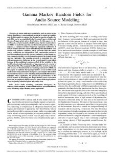
Theoretical framework; Definition, generation and analysis of texture pat terns Model description Figure 1: Neighboring system for a 7 x 7 lattice with a 3 x 3 figure region in the middle. The squares symbolize “connectivity” matrices: the big squares correspond to “figure”, the small squares t o “ground”, and the diamond squares t o “border” matrices.
Julesz used one-dimensional Markov random processes to generate visual textures [ll]. This method showed inherent limitations in generating a larger class of visual patterns. To model the higher order statist i c s of visual textures, Julesz with coworkers proposed a new method that could model the shape of different classes of two-dimensional micropatterns. The method, however, was not purely statistical in nature and the statistical terms, describing the model, were used in the geometrical context of the model. Here we start with the two-dimensional Markov random fields model. This model has also been extensively used as a theoretical model in image analysis of gray scale textures. We assume that spatially local characteristics of the stochastic textures are based on ensemble statistics of the images in contrast to the statistics of cooccurrences in a single image, which is often used in the models of homogeneous, gray scale, textures [6,8]. We assume an n x n lattice t o sample the image space. A neighborhood system N ,over the set of lattice sites S = {SI,s2, ..., sna} defines the set of neighbors N ( s ) C S for every site s E S . A family of random variables X = { X , , s E S} is associated with the network. We assume that each random variable X , takes a value X , = z, from a discrete set of labels 2 , E A = { I 1 , 1 2 , ..., l q ] . N o a priori ordering relation is assumed to apply to the set of labels. We assume, in general, that the set of labels is associated with the set of image filters, locally processing the corresponding features. The configuration space, denoted with R, represents the set of all possible configurations over S:
We consider a class of textures that can be described by a set of parameters - local potentials - of the Gibbs probability distribution. For a given set of local potentials, we assign the Gibbs probability measure over the configuration space SZ:
where ( 2 1 , 2 2 , ..., z,a) E R and the so-called partition function 2 defines the probability structure over the whole configuration space. We consider here two-site local potentials m,t only. Also, we shall not be concerned with the complexity of the computation of the partition function. In the formula above, it denotes the scaling constant. Temperature T parameterizes the family of the Gibbs PDFs in (2.1). The variations in the PDF are smaller for higher temperatures, while the shape of the P D F is the result of increasingly dominant energy terms in the formula as we lower the temperature. Figure 1 shows neighboring system that we use here t o describe unhomogeneous textures. The dots symbolize the sites of the square lattice forming the image. We assume that every site s with four of its neighbors defines the set N ( s ) . The local potentials in m,i define the connections of the two sets of labels between neighboring sites s and t.
270
The “connectivity” matrices in Figure 1 are shown
The temperature parameter controls the degree of the associations for the sets of labels between the neighboring sites, stored in the connectivity matrices. We use the Metropolis algorithm to “relax” the network a t a given temperature. The algorithm governs the asynchronous dynamics by randomly selecting a lattice site and a texture label, and accepts the new label for that site depending on the probability of the resulting configuration. We denote w ( ~as ) the state at the ith iteration for the given temperature, and w‘ as the new state that is the result of applying the selected label at the selected site. Then if we let
as depending on whether the neighboring sites belong
to the same region, and whether they are in the figure or the ground region. In Figure 1, we show three types of connectivity matrices. The “border” matrices are used as a connection between the figure and the ground regions while the basic structure of the regions is described by the “figure” and the “ground” matrices. These matrices are used to locally assign a measure of goodness of particular configuration. As it will be explained in the following section, more favorable combinations of the textural labels at the neighboring sites are associated with relatively lower potentials in the connectivity matrices.
2.2
Generating textures
the new label at the selected site is updated with probability: P(J’+l) = w ’ ) = min(a, 1).
Designing the connectivity matrices in fact we construct:
The number of iterations has to be sufficiently large in order for the network t o reach stochastic equilibrium at a given temperature. Since the network is “relaxed” at some temperature long enough to keep it close to stochastic equilibrium, we are able to compute joint probabilities of the random variables for the neighboring sites. We use joint entropy as a statistical distance measure. The joint entropy for a given temperature can be written as
fized points of an attractor network and,
associations of the two sets of labels between neighboring sites, which reflect dynamics of the network. We consider both kinds of dynamical states, fixed points of the dynamics, and those that are realization of sampling the PDF at different temperatures along the temperature cooling schedule. We consider the equilibrium states for a given temperature. The ensemble statistics is computed t o analyze the generated texture patterns, along with the temperature parameter. Let’s consider w = ( q , z 2 , ..., z,a) E R to be one realization of textural elements on n x n lattice. We can write an energy function E ( w ) for this state as
-H(X,; X,) =
c(lk=l P(x,= zk
xt = z l ) l O g P ( X S= zk 1
xt = X I ) . (2.3)
Visual appearance of generated texture patterns are analyzed in connection with this statistical distance measure for every step of the temperature cooling schedule. We shall show, in the next section, that with this distance measure we can also localize distinct patterns in a composite image from a given ensemble statistics. We illustrate the model with the examples of unhomogeneous (figure-ground) textures - the generalized random stereograms, in the following section.
and the probability of the state according to the Gibbs distribution:
3 We see that states of lower energy have higher probability. We shall show that the temperature acts as a “smoothing” parameter in the sampling process of the PDFs. On higher temperatures, the PDF resembles the uniform distribution and, conversely, the shape of the PDF is dominated more by the set of local potentials on lower temperatures.
Generalized random stereograms
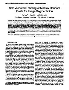
Random dot stereograms was first used by Julesz [lo] to study stereoscopic depth perception, motion perception, and preattentive texture segmentation in human visual system. Figure 2 shows an example of random line stereograms where we use four line elements, instead of black and white dots, as the textural labels. We first explain how the stereo images
271
The stereo pair in Figure 2, when viewed monocularly, lacks any perception of form since it resembles a random configuration of the simple textural elements. However, when fused binocularly, the middle square appears segregated in depth as a result of disparity information, extracted by visual system [lo]. In our example, the high value for the temperature parameter (T = 100) reflects the fact that the configuration in the left image is generated by sampling an approximately uniform probability distribution over the configuration space. We continue now with the description of connectivity matrices used in our example. As we mentioned earlier, we are interested in constructing fixed points of an attractor network, and to observe the texture patterns generated as the equilibrium states at a given temperature. We use the temperature parameter as an objective measure that controls the degree of the associations for the sets of labels between the neighboring sites. Generated texture patterns are also the dynamical states of the network, as they gradually express the structure of the network, stored in the connectivity matrices, along the temperature cooling schedule. We shall not, however, consider here the actual estimation procedures of local potentials for some ensemble of images. In this example we have used the following connectivity matrices:
Figure 2: A stereo pair generated at T = 100.
:
5
’
3
L
4
L
I
5
10
I 11
12
r
1:
15 15 15 15
F,: =
1
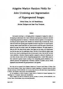
Figure 3: Equilibrium patterns’ statistical measure at T = 100. are formed. We shall analyze the role of the temperature parameter and the statistical distance measure in Figure 3 later.
G,t
=
I
15 15 15
r 15
The image space is formed on a 14x14 lattice. A random process for generating texture patterns produces the left image. We form the right image by a simple manipulation of the left image. We identify the 6x6 square in the middleof the left image and copy its content to the right image, displaced by one column to the right. We fill each neighboring point to the left of the displaced square with a line element which is orthogonal t o the element to its immediate right (first column of the displaced square). This procedure explains how we form the displaced part of the stereo images. The surrounding area in the right image is copied unchanged as that one in the left image.
Bst =
I
15 15
15 15 15 15
15 i 15 15
15 15
15 15 15
15 15
15
(30(
1
15 15 15
15 15 l5 15 15 l5 l5 l5 1 1 5 15 15 15
I
’
’
1
1
’
where F,t, G a t ,B,:, are the “figure”, the “ground”, and the “border” matrices respectively. The rows/columns of the matrices are ordered such that the first row/column corresponds to the horizontal, the second to the oblique, the third to the vertical, and the fourth to the obtuse line element. The “figure” matrix is designed to favor the obtuse line elements in the figure region, while the “ground” matrix is favorable to the oblique line elements in the ground
212
formed figure region with the obtuse line elements whereas the ground region appears of the random structure. The joint entropies of the neighboring sites indicate a general characteristic of the patterns generated at this temperature. Namely, the random structure of the ground region and the progressively stronger associations between the neighboring sites as we go deeper to the middle of the figure region.
We explain this as a consequence of the neighboring structure assigned to this example. The area of summation of the potential terms, in fact, becomes effectively more local in space as we gradually decrease the temperature. This effect becomes visible in the figure region, as it is shown on the texture pattern in Figure 4. Also, we note that the reason for getting unstructured random patterns at very high temperatures (T = 100) is because the area of the summation, for every site of the lattice, is in effect non-local. As we can see in Figure 3, the joint entropy for all of the neighboring sites in the left image reaches an approximately maximal value (log16 = 2.77). In effect, all of the potentials, stored in the connectivity matrices, get averaged out by the sampling process.
Figure 4: A stereo pair generated a t T = 16.608.
3-
ground
12.5 -
2
2I
2-
..z g1.5-
-