A Mechanism for Efficient Debugging of Parallel Programs - Description

A Mechanism for Efficient Debugging of Parallel Programs Barton P. Miller Jong-Deok Choi

Computer Sciences Department University of Wisconsin - Madison 1210 W. Dayton Street Madison, Wisconsin 53706

ABSTRACT This paper addressesthe design and implementation of an integrated debugging system for parallel programs running on shared memory multi-processors (SMMP). We describe the use of flowback analysis to provide information on causal relationships between events in a program’s execution without re-executing the program for debugging. We introduce a mechanism called incremental tracing that, by using semantic analyses of the debugged program, makes the flowback analysis practical with only a small amount of trace generated during execution. We extend flowback analysis to apply to parallel programs and describe a method to detect race conditions in the interactions of the co-operating processes.

evaluated in a test implementation called the Parallel

We borrow terminology from fault tolerant computing community to describe the process of debugging [4]. The first indication that a program is incorrect is usually an externally visible symptom, such the wrong value being printed or the system detecting a fatal problem (such as dividing by zero). This externally visible symptom is called afailure. A failure is causedby an erroneous internal state (called an error) of the program. This error could be an incorrect value for a variable or the program executing in the wrong place (incorrect program counter). An error state is usually preceded by another error state. We can follow this (often long) chain of errors back to the cause. The causeof the initial error is an algorithmic fault in the program. In debugging, these faults are called bugs. Debugging is a difficult job becausethe programmer has little guidance in locating the bugs. To locate a bug that causedan error, the programmer must think about the causal relationships between events in a program’s execution. There is usually an interval between the time when a bug first affects the program behavior and when the programmer notices an error caused by the bug. This interval makesit difficult for the programmerto locate the bug. The usual method for locating a bug is to execute the program repeatedly, each time placing breakpoints (to detect an error) closer to the location of the bug. An easier way is to track the events backward from the moment of detecting an error to the moment at which the bug caused the error, as is done by the @powback analysis[l] approach proposed by Balzer. In flowback analysis, the programmer can see, either forward or backward, how information flowed through the program to produce the events of interest. In this way, the programmer can easily locate bugs that led to the detected errors. This paper is organized as follows. We discuss research related to our work in Section 2, contrasting debugging with repeated execution, trace-baseddebugging, and flowback analysis. Section 3 provides an overview of our strategies for debugging parallel programs. In particular, Section 3 describeshow we divide the process of debugging into several steps and how each of these steps works toward the goal of efficient debugging of parallel programs. We describe in Section 4 the tools that help the user to locate bugs easily. Section 5 describes how to provide these tools in an efficient way and how to make them applicable to parallel programs. We describe a method to detect timing errors in the interac-

1. Introduction Debugging is a major step in developing a program since it is rare that a program initially behaves the way the programmer intends. While most programmers have experience debugging sequential programs and have developed satisfactory debugging strategies, debugging parallel programs has proven more difficult. This paper addressesthe design and implementation of an integrated debugging system for parallel programs running on sharedmemory multi-processors (SW). The major approach described in this paper is to use Balzer’s flowback analysis[l] in providing information on the causal relationships between events in a program’s execution without re-executing the program during debugging. By using semantic analyses of the program, such as inter-procedural analysis[2] and data flow analysis[3], we are able to keep the system overhead in applying flowback analysis low. Our approach also allows for easy detection of race conditions in the interactions of the co-operating processes. This paper describesa method called incremental tracing that makes flowback analysis practical by generating only a small number of traces during execution, and without requiring R-execution of the program during debugging. We extend Rowback analysis to parallel programs. These strategies are being Research supported in part by the National Science Foundation grant CCR8703373, an Office of Naval Research Contract. and an AT&T Graduate Fellowship. Permission to copy without fee all or partof this material is granted provided that the copies are not made or distributed for direct commercial advantage, the ACM copyright notice and the title of the publication and its date appear, and notice is given that copying is by permission of the Association for Computing Machinery. To copy otherwise, or to republish, requires a fee and/ or specific permission. o

I988 ACM O-8979 I -269-l/88/0006/0 135

Language Design and Implementation Atlanta, Georgia, June 22-24, 1988

Program

Debugger (PPD).

tions of the co-operating

work in Section 7.

$1.50

135

processes in Section 6, and summarize

our

2. Related Work

The strategy adopted by us to overcome the above difficulties is to use incremental tracing basedon the idea of need-to-generate. For the user, the effect will be the same as that of generating a trace of every event and state of program during execution, but with far less run time overhead since not every event will actually be traced, The cornerstone of the need-to-generate concept is to generate a small amount of information, called a log, during execution and fill incrementally, during the interactive portion of the debugging session, the gap between the information gathered in the log and the information needed to do the fiowback analysis using the log. By doing so, we can transfer the cost in generating traces from the execution time to the debugging time, and partly to the compilation time since we generate static information during compilation time. We can reduce the run time overhead in producing the log by applying inter-procedural analysis[2] and data flow analysis[3] commonly used in optimizing compilers. Incremental tracing will be described in more detail in Section 5.

There are two major approachesin debugging a parallel program: cyclic debugging (debugging with repeatedexecution of the program) , and debugging with traces of program execution. The main advantage of cyclic debugging [5-71 is that the user need not anticipate the types of bugs that exist in the program until an error is detected. The program can be re-executedto produce the sameexecution behavior. Applying cyclic debugging to parallel programs have a couple of disadvantages. First, executing the entire computation several times while repeatedly setting breakpoints is costly. Second, cyclic debugging requires reproducible program behavior from the program to be debugged and cannot be applied, without special provision by the debugger, to non-deterministic programs. Such non-deterministic program behavior can come from scheduling delays, language constructs such as guarded commanak[8], or from the changes in external environments. A Process accessing a database is a good example of the third case since its execution behavior may depend on the (potentially changing) contents of the databases. The main advantageof debugging with traces [9-121is that the reproducible behavior is not required of the program. This approach can therefore be applied to both deterministic and non-deterministic programs. Its main disadvantage is that generating traces can be costly in time and space. Idealy, we would like hardware support to eliminate the execution cost of tracing. Since this is rarely available, we have to work to reduce the size and cost of the traces. Even with hardware support, it is important to reduce the amount of tracing so as to not go beyond the hardware limitations. Debugging is a difficult job becausethe programmer has little guidance in locating the bugs. To locate a bug that caused an error, the programmer must think about the causal relationships between the events in a program’s execution. Balzer’s flowback analysis[ I] is unique among the trace-basedapproachesin that it is an attempt to directly help the programmer in locating bugs by showing the past flow of program execution and, in doing so, by showing the causal relationship among events. However, Balzer’s suggestion is based on traces of events and sharesthe advantagesand disadvantages of other trace-basedapproaches. Our debugging system provides such direct help with low system overhead. 3. Structural tem

and Functional

Overview

of the Debugging

3.2. Three Phases in Debugging We divide debugging into three phases: a preparatory phase, an execution phase, and a debugging phase. There are two major components in our debugging system: the CompilerlLinker and the PPD Controller. During the preparatory phase, the Compiler/Linker produces the object code, and the files to be used in the debugging phase. While the object code is running in the execution phase, it generates the log to be used in the following debugging phase. When the program halts, due to either an error or user intervention, the debugging phasebegins. 3.2.1. Preparatory

Phase

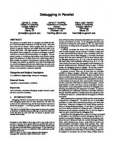
Figure 3.1 shows the preparatory phase, during which the Compiler/Linker produces, along with the object code, the following: 1)

2)

the emulation package that will generate traces during the

debugging phase to fill the gap between the information contained in the log generated during execution phase and the information neededto do flowback analysis; the static program dependence graph that shows the static (possible) data and control dependencesamong componentsof the program;

Sys-

Our approach to debugging parallel programs is to provide direct help in locating bugs without re-executing the program. In providing direct help to locate bugs, we have adopted fiowback analysis[l] to show the actual run time dependences. 3.1. Flowback Analysis and Incremental

Tracing

:----------; : .scJnRa I FILES : 1.-----..--A

Flowback analysis would be straightforward if we were to trace every event during the execution of a program. However, doing so is expensive in time and space. The user needs traces for only those events that may have led to the detectederror. The problem is that there is no way to know what errors will be detected before the execution of the program; either the user has to generate a trace of every event so that the traces wiU not lack anything important when an error is detected, or the user has to re-execute a modified program that generatesthe necessary traces after an error is detected. The first option is expensive, and most often not practical for parallel programs because of unacceptable changes the debugger would introduce in the timing of the interactions between processes. The secondoption is not practicd for programs that lack reproducibility, as is often the casewith parallel programs.

0

COMPILW L.UiKER

-------I-------_ ; ; -0GcfcoDE 1 , ’ r-----1, I E.MuLATlON PACXAOB I ’' I r------

! I 1

I 1 ; PROORAM DATABASE ' 1 " ------I 1 I ' I STATIC 7; ' ] 1I I PROGRAM I ' / '-;_I DEPENDBN(I1 I

------: providedby user L--GE!--J ’ ---. _generatedby compiler ‘- _ _ _ _ _ _ _ _ - - - I

Figure 3.1. The Preparatory

136

Phase

3)

updates the portion of the dynamic graph presented to the user to show the requesteddepcndences. In the secondcase,the PPD Controller directs the emulation packageto generatethe tracesneededto show the requesteddependences. In directing the emulation package, the PPD Controller consults with the static information such as static program dependence graph and program databaseproduced during the preparatory phase. Since not all the events of a program execution are interesting to the user in locating bugs, not all the events will generate traces during the debugging. More details are provided in the next sections.

the program database that contains information on the pmgram text such as the places where an identifier is defined or used.

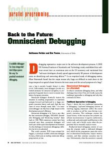
3.2.2. Execution Phase

The object code produced during the preparatory phaseplays a major role in the execution phase. Figure 3.2 shows the execution phase, during which the object code generatesprogram output, and a log that records dynamic information about program execution. The log is used by the emulation package during the debugging phasein generating traces for the flowback analysis. Among the log entries are postlogs, which record the changesin the program state since the last logging point and prelogs, which record the values of the variables that might be read-accessedbefore the next logging point. The postlogs also allow for the restoration of the program state to previous points of program execution. The user could change the values of variables and re-start the program from the samepoint to seethe effect of thesechangeson program behavior.

4. Program Dependence Graphs

Two types of information will be produced by our debugging system as a means of giving direct help in locating bugs: static information based on the program text, and dynamic information based on program execution. The static information consists of the static program dependence graph (also called static graph), the simplified static program dependence graph (also called simplified sfutic graph), and the program database. The simplified static graph is a subset of the static graph, used to show the possible dependences between concurrent events (events belonging to different processes). More details on the simplified static graph are presented in Section 5.5. The dynamic information consists of the dynamic graph and the parallel dynamic program dependence graph (also called parallel dynamic graph). The dynamic graph shows the run time dependences between program components during program execution so that the user can easily locate the bug that causedan error, while the parallel dynamic graph, which is a subset of the dynamic graph, emphasizesthe interactions between processesof a program to help detect timing errors.

3.2.3. Debugging Phase Figure 3.3 shows the debugging phase,during which the PPD Controller plays the major role. In Figure 3.3, the edgestoward the PPD Controller represent the flow direction of the information needed to build the dynamic program dependence graph. The dynamic program dependence graph (also called dynamic graph) shows the run time dependencesamong program componentsand is incrementally built during debugging. In building the dynamic graph, the PPD Controller controls the emulation packageto obtain the necessarytraces. When the debugging phase starts, the PPD Controller presents the user with a portion of the dynamic graph that has the last statement executed being the root of an inverted tree. Since the portion of the dynamic graph presented to the user at any time is small in size (first, there is a practical limit to the size of the graph determined by the screen size; second, it is useless to provide a graph whose size is beyond the user’s grasp), the tracesneededat one time in building a portion of the dynamic graph is also small in size. When the user wants to seethe dependencesof events not seen on the portion of the dynamic graph presentedto the user, the PPD Controller draws a new portion of the dynamic graph that shows the requested dependences. There are two possible caseshere. In the first case, there are sufficient traces already generated to show the dependencesrequestedby the user. In the secondcase,there are not sufficient traces. In the first case, the PPD Controller merely

I I

---. __

---b

: control flow

----+

: informationBow

USER

0

: systemprovided

CL) : compilergenerated

0 : generatedduring debuggingphase ~~-~~~~-~ : generatedduring previousphases

: providedby user . generatedby compiler : generatedby userprogram

Figure 3.3. The Debugging Phase

Figure 3.2. The Execution Phase

137

4.1. Static Information

The dynamic program dependence graph of a program P, denoted as G,, is a directed graph consisting of four types of nodes and four types of edges. The four node types are the ENTRY node, the EXIT node, the singular node, and the sub-graph node. Each node represents a program event (execution of a program component). The four edge types are the flow edge, the data dependence edge, the control dependence edge, and the synchronization

The static graph shows the potential dependencesbetween program components. The static program dependencegraph is a variation of the Program Dependence Graph introduced by Kuck[ 131. Other variations of the Program DependenceGraph have been used for representing programs in vectorizing compilers[lC 171, for integrating program variants(l81, and for debugging programs[l9,20]. Since the Program Dependence Graph shows the possible dependences,we use the name static program dependence graph to distinguish it from the dynamic program dependence graph, which shows the actual dependences.

edge.

The program database contains information that cannot be easily represented by the static graph; for example, where in the program an identifier is defined. The program databasealso keeps the information obtained by semantic analysesof the program, such as the set of variables that may be used or modified when invoking a subroutine[2]. 4.2. Dynamic Program Dependence Graph The dynamic graph shows the causal relations between program events and states during execution. If there are no loops and no conditionals in a program, the dynamic graph of the program will be structurally identical to its static graph. The definition used in this paper is a variation largely borrowed from [ 181,and adaptedto the particular need of showing the run time dependencesbetween program components.

sl s2 s3 s4

+

s5 s6

d=SubD{a,b,a+b+c); if (d>O) sq=sqrt(d); else sq=sqrt(-d); a=a+sq;

___

: datadependence edge - ---.

0 El

:controldependence edge :flowedge

The ENTRY node in a Gp is the point at which control is first transferred into the scope of Gp, and the EXIT node is the point at which control is transferred out of the scope of G,. The singular node correspondsto the execution of either an assignmentstatement or a control predicate such as an if or case statementin the program. When a singular node correspondsto an assignment statement, it is associated with the assigned value. When a singular node correspondsto a control predicate, it is associatedwith the value of the control predicate. The sub-graph node, which is itself a graph (sub-graph), is a way of encapsulating the execution details of several statements. These statements usually correspond to functions or subroutines supplied by the user or the system. The value returned by a function execution is associated with the sub-graph node representing the execution of that function. A flow edge from n; to nj is defined when the event representedby nj immediately follows the event representedby ni during execution; it shows the control flow of the program. A control dependence edge shows a control dependence between two nodes while a data dependence edge shows a data dependence between two nodes[181. The synchronization edge shows the initiation and termination of synchronization events between processes,such as sending and receiving messages. The definition of a synchronization edge is described in more detail in Section 6, in the discussion on detecting timing errors between processes. When a dynamic program dependencegraph either represents the detailed execution of a subroutine or contains a sub-graph node representing the execution of a subroutine, we need to show the mapping between the formal parametersand the actual parameters. We use the symbol “%” to distinguish the passedparametersfrom the regular identifiers. For example, “%l” represents the first parameter, and “%n” representsthe n’th parameter. “%O” is used to represent the returned value if the sub-graph node represents a function execution. Figure 4.1 shows a C program fragment and its dynamic graph at the moment at which statement “~6” is to be executed (indicated by the arrow). Each node contains either an identifier or a predicate expression and a statement number. If the parameter passed to a subroutine is an expression rather than a single variable, we introduce a fictional singular node to accommodatethis. In this figure, the third parameter passed to the function subroutine SubD is an expression, and a fictional node labeled “%3” is introduced. A sub-graph node, which representsa procedure or a function, is itself a graph consisting of nodes and edges. When the user wants to know more execution detail about the sub-graph node, the debugger presents the user a detailed graph corresponding to the sub-graph node.

:singulafnode

: sub-graphnode

Figure 4.1. An Example Dynamic Program Dependence Graph

4.3. Parallel Dynamic Program Dependence Graph The parallel dynamic graph is a subset of the dynamic graph that hides the detailed dependencesbetween local events to better show the dependences between concurrent events. The parallel dynamic graph also allows for identifying race conditions in a

138

program’s execution. The parallel dynamic graph can be thought of as the superstructure of the dynamic graph, since we can build the parallel dynamic graph during program execution and fill in the detailed dependencesbetween local events during debugging. A more detailed description of parallel dynamic graph is given in Section 6, where we present a description of how to order concurrent events and identify race conditions.

the values of the variables belonging to DEFINED(i) at the end of 1,. TO reproduce the same program behavior for interval ri during the debugging phase, we use the program code corresponding to Ii (e-block(i)), the log entries generated during li (LOG(i)), and the sameinput as originally fed to the program during that log interval. We obtain the sets USED(i) and DEFINED(i) by applying data flow analysis[2,21-231 to Ei.

5. Incremental

5.2. Nesting of Log Intervals

Tracing

In this section, we describe incremental tracing in more detail. We first assumethe reproducibility of the program to be debugged. Later in this section, we describe how to make theseoperations possible for parallel programsthat lack reproducibility. 5.1. Emulation

Log intervals can be nested when one subroutine calls another. For example, in Figure 5.2 we assumee-block(j) corresponding to log interval Ii is made up of a subroutine named SubJ. SubJ started at time ti-1 and ended at time ti+z. We also assumee-block(j+l) corresponding to Z,+lis madeup of a subroutine namedS&X. SubK is called at ti (from within Subs) and returns at ti+l. Prelog(j) and postlog are made at ti-1 and li+z, respectively; prelog(j+l) and postlog(j+l) are made at 1; and ti+l, respectively. In this case, we say log interval I,+r is nested inside log interval Ii. When the user is interested in the events between li+, and fi+2, the system retrieves prelog(j) and executes e-block(j) of the emulation package. When the execution of e-block(j) of the emulation package arrives at the point of the subroutine call corresponding to e-block(j+l) (SubK), it updates the program state with posttog(j+l) generated by e-block(jcl) of the object code during the execution phase instead of executing e-block(j+l) of emulation package, and proceedswith the execution until it arrives at the end of e-block(j). The unexecuted portion corresponding to e-block(j+l) will be representedas a sub-graph node in the dynamic graph. If the user wants to know more about the execution detai1 of the sub-graph node, the PPD Controller executes e-block(i+l) of the emulation packageby preparing the initial state with prelog(j+l) from the log file.

Blocks and Logs

As described in Section 3, two types of log entries generated during the execution phase are the prelogs and postlogs. We call the activities to produce such log entries prelogging and postlogging.

The object code generatedby the Compiler/Linker during the preparation phase contains code to generate prelogs and postlogs. By using semantic analysis, we divide the program into numerous segmentsof code called emulation blocks (e-blocks). Each e-block starts with code to generate prelog and ends with code to generate postlog. The prelog consists of the values of the variables that may be read-accessedduring the execution of the e-block. The postlog consists of the values of the variables that may be write-accessed during the execution of the e-block. An e-block is also the unit of incremental tracing during debugging. As will be describedin more detail later in this section, a subroutine is a good example of an emulation block. The i’th prelog and the corresponding postlog generatedduring program execution are called prelog(i) and postlog( respectively. The emulation block that starts with the code to generate prelog(i) and ends with the code to generatepostlog is denoted as e-block(i), and the set of events in e-block(i) is denoted as Ei. The time interval between the prelog and postlog of an e-block is called the log interval and is denoted as I, for the log interval starting with prelog(i). The log entries in log interval ri are denoted as LOG(i). Programs usually contain loops, so a given e-block of a program may have several corresponding log intervals during execution. Figure 5.1 shows the logging points and log intervals. USED (i) is the set of variables that may be read-accessedby Ei. DEFINED(i) is the set of variables that may be write-accessed by Ei. The prelog (i) consists of the values of the variables belonging to USED(i) at the beginning of Ii, and the postlog consists of

time:

*0

fl

12

t3

14

5.3. Object Code and Emulation

Package

The Compiler/Linker generatesthe object code and the emulation package during the preparatory phase. The object code contains the conventional executable code along with code to generate the log entries. The emulation packageis similar to the object code, except that instead of code to generate the log entries, it contains code to generate a trace of every useful event. This section describes how the object code and emulation package are used to

subroutine Cdl

nested log interval

subroutine return

ts

Figure 5.2. A Nested Log Interval

Figure 5.1. Logging Points and Log Intervals

139

subroutine is very large. Though the size of a subroutine has no direct relationship to the time neededto execute it, we can act conservatively to construct several e-blocks out of such a large subroutine.

perform the flowback analysis. Once a program is stopped(due to either an error or user intervention), the PPD Controller locates the last prelog whose corresponding postlog has not yet been generated by the object code. The Controller setsup the initial state for the emulation package using this prelog. Then, the Controller locates the e-block of the emulation package corresponding to this prelog and executes it to generatethe necessarytraces to do the flowback analysis for the events within the e-block. When the flowback analysis is done, the Controller builds a fragment of dynamic graph such as shown in Figure 4.1, and presentsto the user a simplified and abstractform of the dynamic graph. In doing the flowback analysis, the Controller uses the traces generated by the emulation package, the static graph, and the program database (as shown in Figure 3.3). The traces generated in this example correspond only to the log interval of last prelog generated, so the portion of dynamic graph presented to the user is incomplete. After examining the dynamic graph, the user tells the Controller which dependencesare of interest, and therefore which part of the dynamic graph to extend.

There are other casesof e-blocks that are not subroutines, such as the for and while loop constructs. Even though the size may be small, the execution time for these components may be long and may introduce unacceptable time delay in reproducing the traces. E-blocks can be defined for such loops so that the debugging phase can proceed without excessive time spent in re-executing the loops. Still, if the user is interested in the execution details inside such loops, the PPD Controller can re-executethe e-blocks corresponding to the loops. Small and frequently called subroutines can also be a problem. If we make an e-block out of each small subroutine, the amount of logging done during the execution phase may be large enough to introduce unacceptable performance degradation. To avoid this problem, it may be better not to make e-blocks out of the small subroutines that correspond to leaf nodes in the call graph. In this case, the direct ancestor subroutines of these leaf subroutines inherit the USED sets and the DEFINED sets of the leaf subroutines, and perform the logging for the descendentsubroutines.

There are two possible caseshere: first, there may already be sufficient traces generated to show the requested dependences; second, there may not be sufficient traces generated. In the first case, the Controller merely updates the dynamic graph or builds a new fragment of the dynamic graph using traces already generated. In the second case, the Controller locates, with the help of the static graph and the program database,the log interval whose traces are needed to complete the requested part of the dynamic graph. The Controller retrieves the prelog for that interval from the log file and sets up the initial condition for the emulation package e-block. After that, the Controller locates the e-block corresponding to that log interval from the emulation package. The Controller then executes the emulation packagee-block to generatetraces. Finally, the Controller either updates the dynamic graph or builds a new one. The entire processis repeatedas necessaryuntil the user has enough of the dynamic graph to locate their bug. Since only the portions of the dynamic graph in which the user is interested are generated,this is called incremental tracing.

5.5. E-Blocks, Parallel Programs, and Reproducible Behavior So far we have assumedthe reproducibility of the debugged program in describing the operations to perform increment&l tracing. In this section, we describe the possible problems in applying these operations to parallel programs that lack reproducibility and also describe our solutions to the problems. Figure 5.3 contains a subroutine which accessesa global variable named SV. The subroutine also constitutes an e-block. The statement indicated by arrow is the first statement in the subroutine that accesses the variable SV after control transfers to this

ENTRY

int foot) int if

5.4. Constructing E-blocks In this section, we describe how to divide the program into numerous segmentsof code called e-blocks. The only condition for several consecutive lines of code to form an e-block is that the entry point for an e-block must be well defined. Whenever control is transferred from one e-block to another, the control must be transferred to the entry point of the seconde-block. The entry point is where the prelog is made. The postlog is made at the exit point where the control is transferred out of an e-block. One natural candidate for constructing an e-block is the subroutine since the entry and exit points are well defined. The size of the e-blocks is crucial to the performance of the system during the execution and debugging phases. In general, if we make the size of the e-blocks large in favor of the execution phase, the debugging phase performance will suffer. On the other hand, if we make the size of the e-blocks small in favor of the debugging phase, execution phase performance will suffer. While the number of logging points should be small enough so as not to introduce an unacceptable performance degradation during the execution phase, it should also be large enough so as not to introduce unacceptable time delay in reproducing traces during the debugging phase. Consider, for example, the case in which the size of a

--,

a, br ct PI q; (p==...) if (q==...) ( . .. 1 else I /* q */ . ..

1 /" q */ else I /* p */ SV= a+b+SV;

.. . 1 /* p */

) /*

foo3

"/

0 : branchingnode 0 : non-branchingnode

EXIT

Figure 5.3. A Subroutine Accessing a Shared Variable And Its Simplified Static Program Dependence Graph

140

subroutine. In sequential programming, we can make a prelog that savesthe value of SV at the beginning of the e-block. The value of the SV will not be changed until it is first accessedin the statement indicated by the arrow. Therefore, we need at most one prelog and one postlog for each e-block for sequential programming. In parallel programming, them may be more than one process that can accessthe samevariable. If SV is a shared variable, we cannot guaranteethat the value of SV saved at the beginning of the e-block will be the samewhen it is first read-accessedin the e-block, other processes may have changedthe value of SV between thesetwo moments. Reproducible program behavior is not guaranteedand traces generatedduring the debugging phasemay not be the sameas they might have been generated during the execution phase. We need to save more run time information to ensure the reproducibility of parallel programs. Such additional information usually includes the values of the shared variables. The simplified static graph allows us to identify what additional information we have to generate and where in the program we have to generatethat information for paratlel programs. Figure 5.3 shows the simplified static graph for subroutine foo3. The simplified static graph is a subsetof the static graph with only one edge type (flow edge). ENTRY, EXIT, and sub-graph nodes (corresponding to subroutine calls) are the same as in the dynamic graph. However, singular nodes include only control predicates (shown as branching nodes) and synchronization operations such as P and V semaphoreoperations. In our example, we use only the semaphore operations (P and V operations) as synchronization operations. However, this approach can easily be generalized to other synchronization primitives. In constructing the simplified static graph, we are not interested in the other singular nodes and they are not included in the simplified static graph. Thus, the non-branching nodes in the simplified static graph correspond only to ENTRY nodes, EXIT nodes, synchronization operations, or subroutine calls. Branching nodes in the simplified static graph represent the possible control transfers from if or case statements. By partitioning the program into numerous rynch~onization units, the simplified static graph allows us to identify what additional information we need to generateand where in the program we have to generate that information. We define the synchronization unit as follows: Definition 5.1 A synchronization unit consists of all the edgesthat are reachable from a given non-branching node in the simplified static graph without passing through another non-branching node.

The shared variables accessedby a process in a synchronization unit should not be write-accessedby other processeswhile the first process is running inside the synchronization unit. Likewise, the shared variables write-accessedby a process in a synchronization unit should not be mad-accessedby other processeswhile the first process is running inside the synchronization unit. Otherwise, there exists a race condition in accessing the shared variables. If such race conditions do not exist in the user code, no inconsistencies will occur while using the prelog during debugging. If there exists a race condition in an execution instance of a program, even though the log entries am not valid, we can detect and show the causesof the race condition. Further discussion on the method for detecting race conditions in an execution instance of a program appears in Section 6. The prelog generated at the beginning of a synchronization is unique in that it does not have the matching postlog. The general solution might be to construct an e-block out of each synchronization unit. However, doing so would increase the number of log entries to be generated during execution since each e-block generateslogs for the non-shared as well as the sharedvariables. 5.6. Logging and Parallel Programs

There is one log file for each process of a parallel program. Sometimesthe incomplete part of the dynamic program dependence graph presentedto the user may cross the processboundaries when an event of a processis dependentupon an event of a different process. In this case, the PPD Controller locates the second process and its log interval to generate traces necessary to show the requesteddependences. In Section 6, We describehow to locate the secondprocess and how to determine the log interval of the second processto generatetraces. 5.7. Postlogs and Restoration

of Program States

Restoration of the program state to a point of program execution can allow the user to experiment by changing the values of variables to see the effect of such changes on program behavior. The postlogs generatedduring execution will allow for such restoration during the debugging phase. The accumulation of the information carried by all the postlogs from the first postlog, postlog( up to postlog is the same as the information carried by the program state at the time at which postlog is made. Therefore, we can restore the program state by using the postlogs from postlog up to postlog( The program state at any time after that can be restored by using the restored program state and the object code. Such restoration of the program state also solves the problem of halting co-operating processesin a timely fashion[24] since we can easily restore the program state to the interesting point of program execution for each halted process.

Thus the sets (ei, e2, e3, es. e6, e8? egl, (e4, e91, and (e7, e8r es) in Figure 5.3 each constitute a synchronization unit. The values of the shared variables that might be read-accessedinside each synchronization unit correspond to the additional information, and the beginning point of each synchronization unit correspondsto the place the additional information is to be generated. The object code generatesan additional prelog (at the beginning of the synchronization unit) for the shared variables that could be read-accessedinside the unit. There is no corresponding postlog generated for the write-accessedshared variables at the end of the synchronization unit, since the reguhu logs generated at the beginning and end of the e-block contain the values of both shared and non-shared variables. If a synchronization unit does not contain any accessesto a sharedvariable, we do not generatea log entry for that sharedvariable.

6. Parallel Dynamic Graph and Ordering

Concurrent

Events

Ordering concurrent events has two implications. First, it allows the user to see the possible causal reIatior&ips among the concurrent events. Second, it allows for the detection of timing errors in interactions between co-operating processes. In this section, we describe the parallel dynamic graph and describe how it is used to order concurrent events and detect race conditions. The parallel dynamic graph can also help the user analyze the causesof deadlocks.

141

Since an internal edge of a process consists of local events of the process, we can order concurrent events by ordering the internal edgesto which the concurrent events belong. If there is no ordering between two internal edges, there exists a potential race condition, More details on detecting race conditions are given later in this section.

6.1. Parallel Dynamic Graph The parallel dynamic graph is a subset of the dynamic graph that abstracts out the interactions between processeswhile hiding the detailed dependencesof local events. Among the edge types of the dynamic graph, the pa&e1 dynamic graph shows only a modified form of flow edges (called an internal edge), which represent the ordering of local events, and the synchronization edges,which show the initiation and termination of synchronization events. Figure 6.1 contains an example of a parallel dynamic graph with three processes.

6.2. Constructing Synchronization Edges A synchronization edge constructed between two nodes represents a causal relationship between tbe events representedby the two nodes and allows for the partial ordering of the concurrent events. In this section, we describe how to construct syncbronization edges for various synchronization operations such as semaphore operations. In general, we construct a synchronization edge between two concurrent synchronization events if we can identify a causal relationship between the two events.

The parallel dynamic graph of a concurrent program consists of two edge types: the synchronization edgesand the internal edges, and a single node type called the synchronization nodes. 4 synchronization edge from a node to another node representsa causal relationship between the events representedby the two nodes (synchronization nodes) such as sending a messageand receiving the message. All the other nodes of the dynamic graph that do not constitute synchronization nodes in the parallel dynamic graph are called non-synchronization nodes. An internal edge represents a chain of zero or more nonsynchronization nodes. The synchronization node from which either an internal edge or synchronization edge starts is called the start node of the edge, and the synchronization node at which an edge terminates is calIed the end node of the edge. The internal edge corresponds to the actual execution of a synchronization unit described in Section 5. We define the partial ordering of nodes and the edges of the parallel dynamic graph using the “+” operator as foIlows[25]: 1) For any two nodes n 1and Q of the parallel dynamic graph, ni + n2 is true if nz is reachable from n1 by following any sequenceof internal and synchronization edges. 2) For two edges el and e2, el -+ ez is true if nl + n2 is true where n i is the end node of the edge el, and n2 is the start node of the edge ez.

P2

62.1. Semaphores and Synchronization edges We construct a synchronization edge when a V operation of a process unblocks another process. In this case, we create a start node for the V operation and an end node for the event of being unblocked. We also construct a synchronization edge for a V and P semaphoreoperation pair when the V operation changes the value of a semaphorevariable from zero to one and the P operation is the next semaphoreoperation on the same semaphorevariable. In this case,we construct a start node for the V operation and an end node for the P operation. By convention, we do not construct a synchronization edge in the second caseif the V and P operation are done by the same process. Other synchronization operations which can be treated similarly are the monitor and the locking operation[26]. 6.2.2. Messagesand Synchronization Edges When a system uses messagesfor inter-process communication, we defme a synchronization edge by a start node for the event of sending a message, an end node for the event of receiving the message,and a synchronization edge from the sending node to the receiving node. If the sender is blocked until the messageis received by the receiver, we also deline an end node at the sender for the event of unblocking, and a synchronization edge from the receiving node to the end node of the sender. The node at the receiver becomes the end node of the synchronization edge representing the event of sending and receiving a message,and the start node of the synchronization edge representing the unblocking of the senderprocess. In Figure 6.1, node n3 correspondsto a blocking send, while node n4 represents the receiving of the message. Node n5 represents the unblocking event. Edge e4 contains zero events.

P3

6.23. Rendezvous and Synchronization Edges For the Ada rendezvous, we detiue a start node (on the caller process)for the event of calling the rendezvous, an end node (on the callee process) for the event of accepting the call, and a synchronization edge between the two nodes. We also define a start node (on the callee) for the event of exiting from the rendezvous block, an end node (on the caller) for the event of returning from the rendezvous call, and a synchronization edge between the two nodes. The internal edge (on the caller) between the event of calling the rendezvous and the event of returning from the call contains zero number of events since the caller is suspendedduring the call. We can treat the remote procedure call (RPC) in a similar way as we do the rendezvous using two synchronization edges, one for calling to, and another for returning from the RPC. Message

Figure 6.1 An Example Parallel Dynamic Program Dependence Graph

142

semantics that require the receiver to send a special reply message[27] to the senderare similar to the rendezvous.

Second, we have made flowback analysis practical by reducing the amount of traces generated during program execution by transferring this cost from execution time to debugging and compilation time. This transfer of cost is accomplished by using semantic analysis of the debuggedprogram with a technique called incremental tracing.

6.3. Ordering Concurrent Events The parallel dynamic graph allows for ordering concurrent events so that we can identify causal relationship between concurrent events and detect race conditions. In Figure 6.1, assume there exists a shared variable named SV that is write-accessed in edge ei and read-accessedin edge e3. Them are no other accessesto SV. In this case, we can see that there exists a data-dependenceof the second event in e3 on the first event in el and can extend the data dependenceedge of the dynamic graph acrossprocess and processor boundaries by using the parallel dynamic graph. Likewise, we can extend control dependenceedgesacrossthe processand processorboundaries.

Last, we have addressedissues specific to parallel programs those relating to synchronization errors. We can help locate the cause of deadlocks and help detect potential race conditions in processinteractions. The paper provides only an overview of our method for efficiently debugging parallel programs. Many areasrequire more detailed description; someof these areasare currently being investigated and some will be addressedin the near future. We are currently taking a more detailed look at the efficiency and speedof the debugging phase algorithms. One issue is that the representation of the various graph data structures can have a large effect on the speed of the debugging phase algorithms. For exarnple, using bit-mask representationsfor sets of variables (as opposed to a list structure) can have a large payoff. A second (and major) issue is how to detect all potential race conditions in the dynamic graph from a program’s execution. Given a specific edge in a program’s dynamic program dependency graph, it is not difficult to determine if there is another edge that contains a potential read/write or write/write conflict. The problem of finding all pairs of possible conflicting edges is more expensive. We are currently investigating algorithms to reduce the cost of detecting these conflicts. Our long range goal is to build a production quality debugger. To do this, we must consider pointers, separatecompilation, and a user interface. Pointers or aliases make the problem of identifying the used and defined setsof a variable more difficult. One approach is to analyze the program to identify the potential aliases for a given variable [21-23,28,29]. If this analysis produces a small enough set, then these aliases can be included in the used and defined sets. A second approachis to simply record all usesof pointer in the logs. More experience is neededbefore we can evaluate these alternatives Separatecompilation of the program introduces the problem of updating inter-procedural information kept in the program database. We must account for the side effects caused by referencing global variables in a procedure. A debugger that can provide a rich body of information needs an easy-to-useinterface. The graphical information produced by the debugging must be presented in a fotm that is easily understood. This information must be related to information about the program execution state (such as call stacks) and to the program text. The interface must also allow the programmer to easily specify what they want to do. The premise for the ideas described in this paper is to debug parallel programs while minimizing the overhead introduced by the presence of the debugging tools. We have made informal experimental tests of the performance of our techniques. These have been done by hand-annotating programs using the semantic analyses. Our measurementsshow that the tracing addedless than 15% to the program execution time. Though the measurementswere done by using a program with hand-written code to generatelog records, we believe that our prototype Compiler/Liier under construction will generateobject code with similar overhead.

Now, assumethat them also exists another write-accessto SV in edge e2. Here, we cannot tell which of the two events (one in e2 and one in e3) happened first; there exists a race condition. This example shows how we can detect race conditions by using the parallel dynamic graph. 6.4. Detecting Race Conditions As described above, we can detect race conditions using parallel dynamic graph. We will define the race conditions more formally here. As a reminder, note that we have stated that, for two edgese,andea,el+eaistrueifn,+nzistmewherenlistheend node of e1 and n2 is the start node of e2. Definition 6. I Two edgese, and e2 are simultaneous edges if

7 (el + e2) A 7 (e2 -+ el). Dejinition 4.2 The REAL-SET(e,)

is the set of the shared variables readaccessedin the edge ei. The WRITE-SET(ei) is defined similarly.

Definition 6.3

We say two simultaneous edgese, and e2 are race-free if all the following conditions are true: a) WRITESET(e,) n WFXI’l-SET(e2) = 0. b) WRITE-SET(e J n READ-SET(ed = 0. b) READ-SET(e J n WRITE_SET(e2) = 0. In other words, two simultaneous edges e, and e2 are racefree if there exists no read/write conflict or write/write conflict between them. Dejnition

6.4

An execution instance of a program is said to be race-free if all pairs of the simultaneous edgesof the execution instance are race-free. The reason why one can say only that an execution “instance” of a parallel program is race-free is that one cannot tell if a parallel program is race-free unless one considers every possible event (internal or external to the program) that may affect the timing of the process interactions. 7. Conciusion Our approach to efficient debugging of parallel programs has three parts. First, we use flowback analysis to provide direct help to the programmer to debug parallel programs. We have extended flowback analysis to programs consisting of cooperating processes. Flowback analysis has the advantages that it does not require repeatedexecution and that it uses semantic knowledge of the program to help guide the programmerto the location of bugs.

143

8. REFERENCES UI

[20] M. Weiser, “Program Slicing,” IEEE Trans. on Software Engineering SE-10(4)(July 1984).

R. M. Balzer, “EXDAMS - EXtendable Debugging and Monitoring System,” Proc. of AFIPS Spring Joint Computer Conf. 34 pp. 567580 (1969).

PI

K. Cooper, K. Kennedy, and L. Torczon, “The Impact of Interprocess Analysis and Optimization in the R” programming Environment,” ACM Trans. on Prog. Lang. and Syst. S(4) pp. 491-523 (October 1986).

[31

K. Kennedy, “A Survey of Data-flow Analysis Techniques,” Program Flow Analysis: Theory and Applications, S. S. Muchnick and N. D. Jones, Eds., pp. 5-54 Prentice-Hall, Englewood Cliffs, N.J.,

[21] J.M. Barth, “A practical interprocedural data flow analysis algorithm,” Communications of the ACM 21(9) pp. 724-736 (September 1978). [22] J.P. Banning, “An efficient way to find the side effects of procedure calls and the aliases of variables,” Proc. of the SIGPLAN 79 Symposium on Principles of Programming Languages, pp. 29-41 San Antonio, TX, (January 1979). [23] E. Myers, “A precise inter-procedural data flow algorithm,” Proc. of the SIGPLAN

(1981 ).

81 Symposium on Principles

of Programming

Languages, pp. 219-230 Williamsburg, VA, (January 1981).

B. Randell, P. A. Lee, and P. C. Treleaven, “Reliability Issues in Computing System Design,” Computing Surveys lO(2) pp. 123-165 (June 1978).

[24] B. P. Miller and J. D. Choi. “Breakpoints and Halting in Distributed

bl

R. Curtis and L. Wittie, “BUGNET: A Debugging System for Parallel Programming Environment,” Proc. of the 3rd International Conf. on Distributed Computing Systems, pp. 394-399 Denver, (August 1982).

[25] L. Lamport, “Time, Clocks, and the Ordering of Events in a Distributed System,” Communications of the ACM 21(7) pp. 558-565 (July 1978).

[f3

R. D. Schiffenbaur, “Interactive Debugging in a Distributed Programs,” MS. Thesis, EECS Tech Report MITILCSITR-264, M.I.T., (August 1981).

Computer Science 60: Operating Systems, R. Bayer, R. M. Graham, and G. Seegmuller. Eds., pp. 393481 Springer-Verlag. Berlin,

t71

T. J. LeBlanc and J. M. Mellor-Cmmmey, “Debugging Parallel Programs with Instant Replay,” IEEE Trans. on Computers C-36(4) pp. 471-482 (April 1987).

[27] D. R. Cheriton and W. Zwaenepcel, “The Distributed V kernel and its Performance for Diskless Workstations,” Proc. of the 9th SOSP, Operating Systems Review 17(5) pp. 129-140 (November 1983).

@I

E. Dijkstra, “Guarded Commands, Nondeterminacy and Formal Derivation of Programs,” Comm. of ACM 18(8) pp. 453-457 (1975).

PI

P. C. Bates and J. C. Wileden, “High Level Debugging of Distributed Systems: the Behavioral Abstraction Approach,” J. Systems and Softwares 4(3) pp. 255-264 (December 1983).

[28] C. Ruggieri and T. P. Mtntagh, “Lifetime Analysis of Dynamically Allocated Objects,” Proc. of the SIGPLAN 88 Symposium on Principles of Programming Languages, pp. 285-293 San Diego, CA, (January 1988). [29] S. Horwitz, P. Pfeiffer, and T. Reps, “Dependence Analysis for Pointer Variables,” Computer Sciences Tech Report (in preparation}, Univ. of Wisconsin - Madison, (1988).

[41

Programs,” Proc. of the 8th International Conf. on Distributed puting Systems, San Jose, CA, (June 1988).

[26] J. Gray, “Notes on Database Operating Systems,” Lecture Notes in

(1978).

[lOI B. Bruegge and P. Hibbard, “Generalized Path Expressions: A High Level Debugging Mechanism,” Proc. of the SIGSOFTISIGPLAN Symp. on High-Level Debugging, pp. 34-44 Pacific Grove, Calif., (August 1983). F. Baiardi, N. De Francesco, and G. Vaglini, “Development of a Debugger for a Concurrent Language,” IEEE Trans. on Sofhvare Engineering SE-12(4) pp. 547-553 (April 1986). WI R. Snodgrass, “Monitoring Distributed Systems: A Relational Approach,” Ph. D. Thesis, Carnegie-Mellon University, (December 1982). D. J. Kuck, Y. Muraoka, and S. C. Chen, “On the Number of Operar131 tions Simultaneously Executable in FORTRAN-like Programs and Their Speed-up,’ ’ IEEE Trans. on Computers, pp. 1293-1310 (December 1972).

[ill

1141 J. R. Allen and K. Kennedy, ‘ ‘PFC: A Program to Convert FORTRAN to Parallel Form,” TR 82-6, Dept. of Math. Sciences, Rice

University, Houston, Texas, (March 1982). J. R. Allen and K. Kennedy, “Automatic Loop Interchange,” Proc. of the SIGPLAN 84 Symposium on Compiler Construction, pp. 233246 Montreal, Canada, (June 1984).

[I61 K. J. Ottenstein and L. M. Ottenstein, “The Program Dependency Graph In A Software Development Environment,”

Com-

SIGPLAN

Notices 19(5) pp. 177-184 ACM, (May 1984).

[17] J. Ferrante, K. Ottenstein, and J. Warren, “The Program Dependence Graph and Its Use in Optimization,” ACM Trans. on Prog. Lang. and Syst. 9(3) pp. 319-349 (July 1987). [18] S. Horwitz, J. Prins, and T. Reps, “Integrating non-interfering versions of programs,” Proc. of the SIGPLAN 88 Symposium on Principles of Programming Languages, pp. 133-145 San Diego, CA, (January 1988). [19] M. Weiser, “Programmers Use Slices When Debugging,” Communications of the ACM 25(7)(July 1982).

144