A Method to Determine End-Points ofStraight Lines Detected Using

Gideon Kanji Damaryam Int. Journal of Engineering Research and Applications ISSN: 2248-9622, Vol. 6, Issue 1, (Part - 1) January 2016, pp.67-75 RESEARCH ARTICLE

www.ijera.com

OPEN ACCESS

A Method to Determine End-Points ofStraight Lines Detected Using the Hough Transform Gideon Kanji Damaryam Federal University, Lokoja, PMB 1154, Lokoja, Nigeria.

Abstract The Hough transform is often used to detect lines in images, yielding the equations of lines found. It works by transforming a line in a given image to a point in a new transform image while accumulating a measure of the likelihood that a point in the new image corresponds to a line from the original image. The resulting equation of a line describes a line of unspecified length, with no information about the end-points of the actual lines in the image which informed the detection of the line of unspecified length. This paperpresents a method to determine the end-points of the actual lines in the image.The method tracks points from the original image whose transforms led to evidence of lines in the transform image. Consecutive points are then grouped into sub-lines according to whether or not there are enough of them in the group so that they constitute a significant sub-line, and all points in the group are far enough from any other points along the same line, that those other points should not be considered part of the same sub-line.Sample results are shown. Keywords: end-point determination, Hough transform, image processing, robot navigation, self-navigation

I.

Introduction

The processes presented in this paper were developed as part of a system for self-navigation for a mobile robot based on visual data within rectilinear environments such as the inside of a faculty building. A camera mounted on the robot captures an image, and it is processed to determine navigationally important features such as doors and corridors. The robot can then decide its next action while following a higher level program such as “go straight, and turn into the second door on the right”. Features such as corridors and doors are detected by first detecting lines in the image. Detection of lines is accomplished by first detecting lines in the image (of unspecified lengths) using the Hough transform to begin with, and then determining the correct end-points for each line. Detection of lines (whose lengths have not been specified) using the Hough transform is discussed in

details in [1]. Determination of end-points for each line is the subject of this paper and is detailed in 2. Determination of Actual Lines and Sample Results. Before going into that, however, a review of the major highlights of pre-processing of images prior to application of the Hough transform for line detection is presented in 1.1 Summary of Pre-Processing, and highlights of application of the Hough transform is presented in 1.2 Summary of Line Detection with the Hough Transform. 1.1 Summary of Pre-Processing Once an image is captured, it is pre-processed using a scheme detailed in [2]. To summarize that pre-processing scheme, images captured are resized to 128 pixels x 96 pixels. A labelling scheme for pixels in the reduced image is used to specify pixels, which is again presented in Fig. 1.

Figure 1 Image points indexing www.ijera.com

67|P a g e

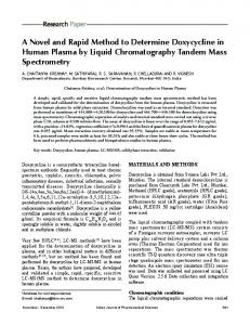
Gideon Kanji Damaryam Int. Journal of Engineering Research and Applications ISSN: 2248-9622, Vol. 6, Issue 1, (Part - 1) January 2016, pp.67-75 Resized images are then converted to intensity images, and edged-detection is done using the Sobel edge-detection operators. Edges resulting are then thinned so that they are mostly a single pixel in

www.ijera.com

thickness. Fig. 2 show a sample of a resized image, and the corresponding thinned image which is ready for line detection using the Hough transform.

Figure 2Sample resized image, and corresponding thinned image(a) Sample resized image (b) Sample thinned image 1.2 Summary of Line Detection with the Hough Transform In [1], a scheme was presented for detection of lines from an image using the straight line Hough transform, for the purpose of vision-based selfnavigation for a mobile robot. A brief summary of the scheme follows: the straight line Hough transform is an image processing technique for detecting lines in images. It has the effect of reducing the search for lines in the original image to a search for a point in a new transformed image, where curves representing lines from the original image intersect in the transform image[3].It works by transforming a line in a given image to a point in a new image while accumulating a measure of the likelihood that a point in the new image corresponds to a line from the original image. This likelihood is informed by the number of points in the original image that would lie on the line if it were drawn from one end of the image to the other. When the transformation is complete, points in the new image can then be subjected to a predefined threshold so that points that are very likely to correspond to lines from the original image can be selected and the original lines identified by reversing the transform. A version of the Hough transform that uses the polar form of the equation of a straight line given in (1) was used and yielded values for the parameters  and  for each line that is considered to be important from the input image.   x cos  y sin  (1)

 and  for each of the important lines found defines the line found using (1), and can be used to reconstruct the gradient-intercept form of the equation of the line using: (2) y   cosec  x cot obtainedby rearranging (1). This gives the gradient as www.ijera.com

m  ( cot ) , .

. and the intercept on the y axis as . c  cosec

.

(3)

.

.(4)

(2) describes the orientation and location relative to the y-axis, of the line found, but it does not say anything about the length of the line or its endpoints. This paper presents a method to determine the endpoints of lines. 1.3 Other Approaches to End-Point Determination Other methods have been proposed for determining endpoints. For example, [4] suggestsa method where a search corridor of width of 5 pixels is set up in the edge image with the line defined by equation (1) as the centre of the corridor. Coordinates of edge points found within this corridor are stored and the points are deleted from the edge image. If points found do not account for up to 50% of the accumulation corresponding to that line, the search corridor is rotated by angles up to the error in  . Edge points previously deleted are restored and the search is started all over again. A problem with this approach is, if an edge pixel has contributed to the accumulation for more than one line, it is only accounted for once and deleted, and there is the possibility that points which should genuinely be on a line are not reported to be on it. This can affect the accuracy of the endpoints and lengths returned eventually. [4]propose to search for points in descending order of the transform strengths of line segments as a way to minimise this effect, but even this proposal does not eliminate the possibility. [5]suggests other approaches: 1. application of corner detection methods and estimating line lengths from corners 2. setting up of four further accumulator arrays to hold the x and y values of the most north-

68|P a g e

Gideon Kanji Damaryam Int. Journal of Engineering Research and Applications ISSN: 2248-9622, Vol. 6, Issue 1, (Part - 1) January 2016, pp.67-75

3.

easterly and the most south-westerly ends of the lines at the time of transformation setting up four further accumulator arrays, storing values for wx ,

wy , (wx )

2

and

(wy ) 2 and working out ends of line using

 wx  2   ( wx) w w the

x

  wx     w    coordinates 2

 wy  2   ( wy ) w w

2

2

  wy     w   

for and 2

for

the y coordinates. ( w is the value with which the main accumulator array is incremented for each ( x, y ) ) Problems with the first suggestion include the complications and computing overheads related to corner detection. The second suggestion is the easiest to implement but has the drawback that determination of end points for lines with a northwest – southeast orientation has very low chance of succeeding. The third suggestion assumes that the points are spread evenly across the line, but this is not necessarily always the case, and the results can be very misleading.

II.

Determination of Actual Lines and Sample Results

The Hough transform scheme summarized in 1.2 yields the  and  values of the most significant lines from the original image. The equations of the lines required can be obtained using equations (2), as discussed in 2 Background earlier. However the lengths of the lines they came from are still not defined. Endpoints need to be determined for genuine lines. This work proceeds by tracking all points which contributed to each of the peaks found, and find out if they make up any valid sub-lines. Here a sub-line, SL, say, for a line L, can be defined as a shorter line that is contained in L, i.e., all points that make up SL also contribute to making up L. A valid sub-line is a sub-line which meets these further criteria: 1. It must reach a certain minimum number, Lm in ,of pixels in length 2. It must have a minimum separation of a certain number of pixels, S m in , from any other line segment on the same infinite line, otherwise the two lines segments are labelled as one line segment. Endpoints of sub-lines can then be worked out from the points that make them up.

www.ijera.com

www.ijera.com

Determination of values for the parameters Lm in and

S m in for these criteria is discussed in 2.1 Values of Parameters for Criteria for Valid Sub-lineswhich follows shortly. The algorithm for finding valid sub-lines, has two main components which are: 1. Determine which points contributed to each subline 2. Find the number of points on each sub-line, noting which ones have Lm in points or more, and are at least S m in pixels away from other points or lines. They are given in 2.2 Assigning Contributing Points to Sub-line, and 2.3Selection of Valid SubLines.An algorithm for determining endpoints for each valid sub-line is then discussed in 2.4 Endpoints and Length Determination. 2.1Values of Parameters for Criteria for Valid Sub-lines The minimum distance for sub-lines, Lm in , was set at 8 because from studying typical images, it is a reasonable general minimum length for significant features in an image. Images in this work are 128x96 pixels in size. The selection of this image size is discussed in [1]. Consider the images in Fig.3. Fig.3a shows a typical image of a corridor magnified 2 times for clarity, and Fig.3b shows a thinned version of it magnified 4 times also for clarity. Fig.3c shows the area enclosed by the blue dashed box of Fig.3b further magnified 2 times. For the purpose of this work, lengths such as the width of the brown door area circled in red on the right of the door are about the smallest lengths of features that might be significant. Any feature shorter than that is probably too insignificant from that distance. As the robot moves nearer to objects, those objects of-course become larger, and have a higher chance of getting detected if they are important. The width of the brown bit is represented by a length of approximately 8 pixels as can be estimated by closely examining Fig.s3b and 3c. S m in was chosen in a similar manner. Within the area surrounded by the green cycle, there is what would be to a human observer, a separation between two features. In Fig.3b, the two features appear as one continuous line. The Hough transform would pick them up as single line as depicted in Fig.3d. The separation between them is 3 pixels, as can be seen by studyingFig.3b and Fig.3c. It can be argued that a separation of about that much is about the least that should reasonably be expected to be identifiable. Any separation less than that is likely to be a crack in a genuine line. Examples of such are circled in red in Fig. 3c. 69|P a g e


www.ijera.com

www.ijera.com

70|P a g e


www.ijera.com

Figure 3Parameters for selection criteria for valid sub-lines (a) A typical image showing smallest significant length of line segment and separation between 2 line segments on the same line (b) Thinned version of Fig.3a image (c) Enlargement of the area of Fig. (b)image enclosed in blue dashed rectangle (d) Single line found by the HT consisting of multiple sub-lines

2.2 Assigning Contributing Points to Sublines The first bit of the sub-line determination algorithm is presented here. Its purpose is to determine which sub-line each point belongs to. The steps taken follow: 1. Set up a variable, LN (line number) say, to count the number of lines found and initialise it to 0 2. Set up an array LI (line-in) of size CP (contributing points) to hold information about which line each point in the significant line found from the Hough transform application of [1], is in. CP is the number of points which contributed to that line. 3. Set up two types of pivot indices. The first, LP , the line identification pivot, which tracks the first point of the current line, and the second, DP , the distance pivot, which tracks the point on the line that is currently being compared with other points to see if they are on the line. Initialise both LP and DP to 0 4. Set up a distance threshold, dT . This is the smallest distance between consecutive contributing points which implies that the two points are on separate sub-lines (on the same www.ijera.com

5.

6.

7. 8.

9.

infinite line). In this work, this is set to 3 as discussed earlier in this section For all points p which contributed to the infinite line under consideration, initialise the LI array to -1 (or any number which will not arise naturally) While LP , the pivot, is less than CP , the number of points which contributed to the line under consideration, do 7 to 16 If LI LP  1 , i.e. if the line that point LP is in has not yet been determined, do 8 else do 17 Assign the line-in array element for the current pivot LI LP to LN ( a fresh line ID). Increase

LN by 1 to make it ready for the next fresh line. Set DP , the distance pivot to LP the line label pivot Set p to LP  1

10. If LI p  1 , i.e. if point

p has not been

processed already, do 11 else do 15 11. Obtain n DP , the index of DP the distance pivot in the original image, using nDP  CPADP . ( CPA is the array which holds indices of contributing points for lines, i.e. points from image space which contributed to each line. It is set up during implementation of the Hough 71|P a g e

Gideon Kanji Damaryam Int. Journal of Engineering Research and Applications ISSN: 2248-9622, Vol. 6, Issue 1, (Part - 1) January 2016, pp.67-75 transform). Determine x DP and y DP , the coordinates of the point in image space using:

1.

Set up an array LL (line length) of size LN to hold the length of each possible subline in each significant line found from the processes discussed to this point. LN is number of lines (groups of points lying on a line with 3 or more pixels separation from all other points along the same line) found.

2.

Determine the length

xDP  (nDP %128  64 ) y DP  (47  nDP / 128 ) 12. Obtain n p , x p and y p in a similar way for p , the point being checked against DP using:

n p  CPA p x p  (n p %128  64 )

y p  ( 47  n p / 128 ) 13. Determine the distance, d, between the two points using:

d 14.

x

 x p    y DP  y p  2

DP

2

If d  dT place as line pivot

LI p  LI LP and make

p on the same sub-line

LP ,

p the distance pivot

DP  p

p by 1

15.

Increase

16. 17.

Go back to 10 if p has not reached CP Increase pivot LP by 1 and go back to 6

2.3

Selection of Valid Sub-Lines

To check for „validity‟ of sub-lines, the second component of the sub-line determination algorithm of 2. Determination of Actual Lines, the following steps are taken:

www.ijera.com

3.

LL l for all lines l ,

0  l  LN , by counting the number of points which make it up. For all lines which have 8 points or more, i.e., LL  8 , assign a unique ID, note the number of points which make up the line, and note the ID numbers of all the points which make up the line

2.4Sample Result of Sub-Lines Determination Algorithm The images in Fig.4 which follows illustrate the results of the sub-lines determination algorithm. Fig.4a shows a typical thinned image, 4b shows the lines found after application of the Hough transform and post processing to the point of butterfly filter application. There were 49 of them. Fig.4c shows the sub-lines found by this algorithm. 40 sub-lines were found altogether. Fig.4c was set up by plotting individual points that contributed to each sub-line. The first sub-line found on a line segment is coloured red. If there is a second sub-line, it is coloured blue, and if there is a third one, it is coloured green. (No lines encountered in the course of the work had more than 3 sub-lines.)

Figure 4Result of sub-line detection algorithm www.ijera.com

72|P a g e

Gideon Kanji Damaryam Int. Journal of Engineering Research and Applications ISSN: 2248-9622, Vol. 6, Issue 1, (Part - 1) January 2016, pp.67-75 (a) Typical thinned image input to algorithm 5.8 for finding sub-lines (b) Lines found with the Hough transform (c) Sub-lines found (d) Lines from which sub-lines were found Fig. 4d shows the lines from which the sub-lines were extracted. There were 30 of them. Infinite lines

Line ID

Number of SubLines

0

1

1

1

2

2

3 4 5 6

1 1 1 2

7

1

8

2

9

3

10

2

11

2

12

2

13 14

1 1

15

1

16

1

17 18

1 1

19

2

20

1

www.ijera.com

which do not have any suitable sub-lines are dismissed as false recognitions. In this example, 19 lines were dismissed for this reason. Table 1 contains further details about the number of sub-lines found in each line, and the points which made up each subline.

Table 1 Details of Results of Sub-Lines Determination for a Sample Image Number of Points in IDs of Contributing Points for Sub-Line Sub-Line(s) 1781 1909 2037 2165 2293 2421 2549 2677 2806 2934 3062 3190 3318 3446 17 3574 3702 3830 9 9585 9842 9970 10098 10226 10354 10482 10610 10738 11 202 330 459 716 845 973 1102 1230 1359 1487 1616 14 2773 2902 3030 3159 3416 3544 3673 3801 3802 4059 4187 4316 4573 4701 10 5078 5206 5334 5462 5591 5719 5847 5975 6103 6231 8 5078 5206 5334 5462 5591 5719 5847 5975 10 3019 3147 3275 3403 3532 3660 3916 4044 4173 4301 12 2506 2634 2891 3019 3147 3275 3532 3660 3916 4044 4173 4301 9 8531 8787 8915 9043 9171 9428 9556 9684 9812 4571 4572 4573 4575 4576 4578 4580 4581 4582 4583 4585 4586 4587 4589 21 4590 4592 4594 4595 4597 4598 4599 8 1867 2123 2251 2380 2508 2636 2764 2892 10 9552 9681 9809 9937 10193 10321 10449 10577 10833 11089 12 2001 2129 2257 2385 2513 2641 2769 2897 3025 3153 3281 3409 3793 3921 4049 4177 4305 4433 4561 4689 4817 4945 5073 5201 5329 5457 34 5585 5713 5841 5969 6097 6225 6353 6481 6609 6737 6865 6993 7249 7377 7505 7633 7761 7889 8017 8145 9169 9297 9425 9553 9681 9809 9937 10193 10321 10449 10577 10833 20 11089 11217 11345 11473 11601 11729 11857 11985 2772 3028 3156 3284 3412 3540 3668 3796 3924 4052 4180 4308 4436 4564 36 4692 4820 4948 5076 5204 5332 5460 5588 5716 5844 5972 6100 6228 6356 6484 6612 6740 6868 6996 7124 7252 7380 12 9428 9556 9684 9812 9940 10068 10196 10324 10452 10580 10836 10964 8652 8654 8773 8774 8775 8777 8779 8896 8897 8898 8899 9017 9018 9019 30 9020 9021 9022 9140 9141 9142 9143 9144 9261 9263 9265 9266 9384 9385 9386 9387 9505 9506 9507 9508 9509 9625 9626 9627 9628 9629 9630 9631 9747 9748 23 9749 9750 9751 9752 9869 9870 9871 9872 9873 10 5719 5847 5975 6103 6231 6359 6487 6615 6743 6871 9 9428 9556 9684 9812 9940 10068 10196 10324 10452 11 5591 5719 5847 5975 6103 6231 6359 6487 6615 6743 6871 14 9626 9627 9628 9629 9630 9631 9632 9746 9747 9748 9749 9750 9751 9752 9280 9281 9282 9283 9401 9403 9404 9405 9406 9523 9525 9526 9527 9645 29 9646 9647 9649 9766 9767 9768 9769 9770 9771 9889 9890 9891 9892 10012 10015 7260 7388 7516 7644 7772 7900 8028 8156 8284 8412 8668 8796 8924 9052 17 9180 9308 9564 12 9765 9766 9767 9768 9769 9770 9771 9772 9889 9890 9891 9892 10 10071 10327 10455 10583 10711 10839 10966 11222 11350 11478 12 4573 4701 4957 5085 5213 5341 5469 5597 5725 5853 5981 6109 8028 8156 8284 8412 8668 8796 8924 9052 9180 9308 9564 9692 9820 9948 19 10076 10204 10332 10460 10588 13 5994 6122 6250 6378 6506 6635 6763 6891 7019 7147 7275 7403 7531

www.ijera.com

73|P a g e

Gideon Kanji Damaryam Int. Journal of Engineering Research and Applications ISSN: 2248-9622, Vol. 6, Issue 1, (Part - 1) January 2016, pp.67-75 21 22 23 24

1 1 1 1

8 8 8 8

25

2

26 27

1 1

8 11 10

28

1

19

29

1

19

6635 6763 6891 7019 7147 7275 7403 7531 246 501 629 757 885 1140 1268 1396 759 887 1015 1143 1270 1398 1526 1654 7282 7410 7538 7666 7794 7922 8050 8178 6386 6514 6642 6770 6898 7026 7154 7282 7410 7538 7666 7794 7922 8050 8178 9842 9970 10098 10226 10354 10482 10610 10738 2806 2934 3062 3190 3318 3446 3574 3702 3830 4086 4214 3832 4088 4216 4344 4472 4727 4855 4983 5111 5367 2806 2934 3062 3190 3318 3446 3574 3702 3830 4086 4214 4342 4470 4598 4855 4983 5111 5367 5495 2810 2938 3066 3194 3322 3450 3578 3834 3962 4090 4218 4474 4602 4730 4986 5114 5242 5498 5626

15

2.5 Endpoints and Length Determination Up till this point, valid sub-lines have been found and are defined by a unique identification number, the line they came from and the identification numbers (or indices) of their contributing points CP, i.e. the points that make them up. A sample of these details for the image in Fig.4 is given in Table 1. Endpoints can now be determined. The scheme which follows was used by this work. At the core of it, it involves: 1. Pick up the index of the first point of a subline and use it as a pivot point:

x0  ID %128

y0  ID / 128 x pivot  x0 y pivot  y0 2.

Initially set the first point to be the farthest point on both sides of the line

mxDistIndex  ID mnDistInde x  ID

and the maximum and minimum distance to 0

mxDist  0 mnDist  0 For all other points i which contributed to

3. the sub-image, do 4 to 8 4. If the gradient of the line is less than or equal to 1 do 5 and jump to 7 else do 6 5. Calculate the horizontal distance from the pivot point, i.e. the first point, to point i using

dist  x pivot  xi 6.

Calculate the vertical distance from the pivot point, i.e. the first point, to point i using

dist  y pivot  yi 7.

If the distance is higher than the currently stored maximum distance, use it to replace the currently stored maximum distance, and www.ijera.com

www.ijera.com

8.

store its index as the index of the maximum distance if dist  mxDist then mxDist  dist ; mxDistIndex  index If the distance is lower than the currently stored minimum distance, use it to replace the currently stored minimum distance, and store its index as the index of the minimum distance if dist  mnDist then mnDist  dist ; mnDistIndex  index

Steps 1 to 8 are done for each sub-line and result in the indices of the extreme points of the sub-line being stored in mxDistIndex and mnDistIndex . The sequence of steps finds the highest and the lowest distance from the first point. If the first point is itself at one of the extreme positions of the sub-line, then one of the distances will be 0, otherwise, one will be positive and the other will be negative. Step 4 is necessary to ensure that the distance is calculated in a direction such that the kind of distance – vertical or horizontal – chosen will result in the most noticeable distances along the line. There is no point working out horizontal distance between points on a vertical or near vertical line for example as they will all be about the same. Once the indices of the points are known, their x and y coordinates can be worked out using the integer operations:

x mxDist  mxDistInde x%128 .

.

.

(5a)

y mxDist  mxDistInde x / 128 .

.

.

(5b)

xmnDist  mnDistInde x%128 .

.

.

(5c)

y mnDist  mnDistInde x / 128 . . . (5d) The length, L of the sub-line, if desired, can also be worked out using: 74|P a g e


L

www.ijera.com

xmxDist  xmnDist 2   ymxDist  ymnDist 2 (6) III.

Conclusion

A scheme has been presented to determine sublines of lines (of unspecified lengths) detected using the Hough transform by tracking the points which contributed to the detection of that line (of unspecified length) by the Hough transform, and analysing groups of consecutive points along the line to see which groups have enough points to be considered valid sub-lines, while being sufficiently far from any other point or groups of points along the same line. A method to determine their end-points has also been presented The choice of parameters to constitute criteria to decide if a line is long enough to be important, or far enough from other points to be considered a separate sub-line, depends on the specific application, and the size and nature of images involved.

Acknowledgement This paper discusses work that was funded by the School of Engineering of the Robert Gordon University, Aberdeen in the United Kingdom, and was done in their lab using their robot and their building.

References [1]

[2]

[3]

[4]

[5]

G. K. Damaryam, A Hough Transform Implementation for Line Detection for a Mobile Robot Self-Navigation System, International Organisation for Scientific Research – Journal of Computer Engineering, 17(6), 33-44, 2015 G. K. Damaryam and H. A. Mani, A Preprocessing Scheme for Line Detection with the Hough Transform for Mobile Robot Self-Navigation, In Press, International Organisation for Scientific Research – Journal of Computer Engineering, 18(1), 2016 A. O. Djekouneand K. Achour, Visual Guidance Control based on the Hough Transform,IEEE Intelligent Vehicles Symposium, 2000. V. F. Leavers,Shape Detection in Computer Vision Using the Hough Transform(London: Springer-Verlag, 2013). A. Low,Introductory Computer Vision and Image Processing,(London, United Kingdom: McGraw-Hill Book Company, 1991).

www.ijera.com

75|P a g e