A Methodology Based on Formal Methods for Predicting the Impact of ...

A Methodology Based on Formal Methods for Predicting the Impact of Dynamic Power Management ? A. Acquaviva, A. Aldini, M. Bernardo, A. Bogliolo, E. Bont`a, E. Lattanzi Universit` a di Urbino “Carlo Bo” Istituto di Scienze e Tecnologie dell’Informazione Piazza della Repubblica 13, 61029 Urbino, Italy {acquaviva,aldini,bernardo,bogliolo,bonta,lattanzi}@sti.uniurb.it

Abstract. One of the major issues in the design of a mobile computing device is reducing its power consumption. A commonly used technique is the adoption of a dynamic power management policy, which modifies the power consumption of the device based on certain run time conditions. The introduction of the dynamic power management within a battery-powered device may not be transparent, as it may alter the overall system behavior and efficiency. Here we present a methodology that can be used in the early stages of the system design to predict the impact of the dynamic power management on the system functionality and performance. The predictive methodology, which relies on formal methods to compare the properties of the system without and with dynamic power management, is illustrated through the application of its various phases to a simple example of power-manageable system.

1

Introduction

Reducing the power consumption is a fundamental criterion in the design of battery-powered devices typical of modern mobile embedded systems. Significant power savings can be achieved at run time through the application of dynamic power management (DPM) techniques [3], i.e. techniques that – based on run time conditions – modify the power consumption of the devices by changing their state or by scaling their voltage or frequency. The approaches to DPM proposed in the literature have been classified into deterministic schemes, predictive schemes, and stochastic optimum control schemes. The schemes of the first class schedule the shutdown periods at fixed time instants, possibly depending on the occurrence of some event. Instead, the schemes of the second class attempt to predict the device usage behavior in the future based on historical data patterns. Finally, the schemes of the third class make probabilistic assumptions – based on observations – about usage patterns to formulate an optimization problem. ?

Co-financed by Regione Marche within the CIPE 36/2002 framework.

Whatever scheme is adopted, the introduction of the DPM within a mobile computing device may have a non negligible impact on the overall system functionality and performance. It is therefore of paramount importance to assess such an impact before the DPM is introduced, in order to make sure that the system behavior will not be significantly altered and that the quality of service will not go below an acceptable threshold. This objective can be achieved by following a methodology that helps predicting the effect of the DPM through the comparison of the functional and performance characteristics of the system without and with DPM. Since it should be applied in the early stages of the system design – in which a high level of abstraction is admitted that favors the task of verifying properties – the predictive methodology can take advantage of formal description techniques, like e.g. stochastic process algebras [7] and stochastic Petri nets [2], as well as formal analysis techniques, like e.g. equivalence checking [11] and model checking [10]. This paper describes and discusses a formal methodology introduced by the same authors for predicting the impact of the application of a DPM strategy [1]. The rest of the paper is organized as follows. In Sect. 2 we present an introduction to DPM including a brief survey of the most frequently adopted techniques. In Sect. 3 we discuss the methodology based on formal methods to predict the impact of the DPM on the system functionality and performance. After recalling in Sect. 4 a particular specification language that provides all the ingredients that are needed to support the predictive methodology, an application of the methodology itself to a simple power-manageable mobile device is illustrated in Sect. 5, 6, and 7. Finally, in Sect. 8 we draw some conclusions.

2

Dynamic Power Management

Electronic systems are designed to deliver peak performance, but they spend most of their time executing tasks that do not require such a performance level. For instance, hand-held personal digital assistants are mainly used to run interactive applications (such as personal organizers and text editors) whose main task is capturing sparse input events, while cellular phones are reactive systems that are usually idle waiting for incoming calls or user commands. In general, electronic systems are subject to time-varying workloads. Since there is a close relation between power consumption and performance, the capability of tuning at run time the performance of a system to its workload provides great opportunity to save power. Dynamic power management (DPM) techniques dynamically reconfigure an electronic system by changing its operating mode and by turning its components on and off in order to provide at any time the minimum performance/functionality required by the workload while consuming the minimum amount of power. The application of DPM techniques requires i) power-manageable components providing multiple operating modes, ii) a power manager having run-time control of the operating mode of the power-manageable components, and iii) a

DPM policy specifying the control rules to be implemented by the power manager. The simplest example of power-manageable hardware is a device that can be dynamically turned on and off by a power manager that issues shutdown and wakeup commands according to a given policy. When turned on, the device is active and provides a given performance at the cost of a given power consumption. When turned off, the device is inactive, hence provides no performance and consumes no power. The workload of the device is a sequence of service requests issued by a generic client. If the workload keeps the device busy for 30% of time, up to 70% of energy can be saved by turning the device off during idle periods. Under the assumption that the device can be switched on and off instantaneously at no cost, the maximum power saving can be achieved without performance penalty by means of a greedy policy turning off the device right after each service accomplishment and turning it on upon each incoming service request. In all cases of practical interest, however, shutdown and wakeup transitions have non-negligible costs both in terms of energy and in terms of time. Transition costs make the design of DPM policies a non-trivial task for two main reasons. First, a shutdown can be counterproductive if the idle period is not long enough to compensate for the transition energy. Second, if a service request is issued when the device is inactive, the wakeup time adds a delay to the service time that may cause an unacceptable performance degradation. In practice, transition costs limit the actual exploitability of low power states and make it necessary to predict user idleness to take DPM decisions. In the rest of this section we show how to describe a DPM system as a power state machine, we provide a formal definition of exploitability of a low power state, we discuss the issue of workload prediction, we briefly outline typical DPM strategies, and we introduce a simple case study that will be used throughout the paper. 2.1

Power State Machine

As far as DPM is concerned, a power-manageable system (or component) can be represented as a power state machine (PSM). Power states are operating modes characterized by average performance and power values. They are called active if they provide positive performance, inactive otherwise. Transitions among power states are characterized by their costs (transition time and energy) and triggered by DPM commands or service requests. Many power-manageable components have only two power states and can be represented by a PSM like the one shown in Fig. 1.a). Transitions from the active state (on) to the inactive state (off) are triggered by a shutdown command issued by the power manager, while wakeup transitions are triggered by incoming service requests issued by the client. Fig. 1.b) shows a more complex PSM with multiple active and inactive states, representing a server with two processing units. The server is sensitive to shutdown commands (sd) when idle. Wakeup transitions are triggered by incoming

idle on2

2:0

busy1 eos sr

2:1

sd

on1

sd

sr off

1:0

sleep sleep

busy2 2:2

sr

sd on

eos sr

eos sr

1:1

sr sr

sd off

off

(a)

(b)

Fig. 1. a) Power state machine of a two-state power-manageable system; b) power state machine of a power-manageable system with 5 active states (labeled x:y, where x is the number of active servers and y is the number of requests under processing) and 2 inactive states (sleep and off), representing a server with 2 CPUs

service requests (sr). The active states span the tradeoff between power and performance, while the inactive states provide different tradeoffs between stand-by power and wakeup cost. 2.2

Exploitability of Low Power States

We now define and discuss the exploitability of the inactive states of a powermanageable component. Since any component needs to be active to deliver its service, the inherent cost of putting it into an inactive state can be computed as the sum of the costs of the shutdown and wakeup transitions needed to enter and exit the inactive state starting from the closest active one: Ttr = Tshutdown + Twakeup

Ptr =

Tshutdown · Pshutdown + Twakeup · Pwakeup Ttr

(1)

(2)

where Ttr is the overall transition time and Ptr is the average transition power. If the transition power is greater than the active power (Pon ), the transition to the inactive state provides a power reduction if and only if the time spent in the inactive state is long enough to compensate for the extra transition power. If this is not the case, the transition is counterproductive. The minimum idle period that makes it convenient to go to the inactive state is called break-even time (Tbe ) and can be computed as follows:

Tbe = Ttr + Ttr ·

Ptr + Pon Pon − Pof f

(3)

The break-even time of an inactive state is closely related to its exploitability: An inactive state is exploitable if and only if the workload contains idle periods longer than its break-even time. Notice that the break-even time is a property of the inactive state independent of the workload, while the exploitability depends both on the break-even time and on workload statistics. For a given workload, the lower the break-even time of an inactive state, the higher its exploitability. The average power saved by entering an inactive state (off) during an idle period of length Tidle > Tbe can be expressed as: Psaved,of f (Tidle ) = (Pon − Pof f ) ·

Tidle − Tbe Tidle

(4)

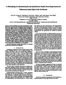
Needless to say, the lower the break-even time and the lower the power consumption of the inactive state, the higher the energy saving. If multiple inactive states are available, their exploitability and energy saving need to be evaluated at each idle period. Given two inactive states (off1 and off2) of the same component, if off2 has a longer break-even time and a higher power consumption than off1 we say it is dominated by off1 since off1 is always more convenient than off2.

1Pon OFF1: Tbe = 10, Poff = 0.6Pon OFF2: Tbe = 5, Poff = 0.5Pon OFF3: Tbe = 7, Poff = 0.3Pon OFF4: Tbe = 15, Poff = 0

0.9Pon

Average power

0.8Pon

0.7Pon

ON

0.6Pon

OFF2

0.5Pon OFF3 0.4Pon OFF4 0.3Pon

0

10

20

30

40

50

Tidle

Fig. 2. Average power consumption during an idle period of length Tidle achieved by exploiting four different inactive states

Fig. 2 shows the average power consumed by a system during an idle period of length Tidle under the assumption that its low power states are carefully exploited by an ideal power manager. The four curves refer to the four different inactive states of the system. Notice that for Tidle < 5 no inactive state is exploitable and the average power consumption is Pon . For larger idle periods, inactive states can be exploited to reduce power consumption. Fig. 2 clearly shows that the relative energy efficiency of the inactive states depends on Tidle . In particular, for 5 < Tidle < 12 the best choice is off2, for 12 < Tidle < 34 the best choice is off3, for Tdile > 33 the best choice is off4. The inactive state off1 is never the best choice since it is dominated by off2, which has a lower power consumption and a shorter break-even time. The inactive states of properly designed power-manageable components do not dominate each other, rather, they provide different tradeoffs between breakeven time and power consumption. Given a power-manageable system, an ideal power manager achieves the best energy saving from each idle period. To this purpose, it needs to evaluate the exploitability and energy savings of all inactive states, then chooses the exploitable state (if any) providing the highest savings. In addition, if no performance degradation is tolerated, the power manager needs to wake up the system right in time to serve the next service request. Similar considerations apply to the choice of the best active state to be used to serve each request. Referring, for the sake of simplicity, to the two-state power-manageable system of Fig. 1.a), the average power saving achieved by the ideal power manager without impairing performance can be expressed by: Psaved,of f = (Pon − Pof f ) ·

avg Tidle>T − Tbe be · (1 − FTidle (Tbe )) avg Tidle

(5)

avg avg where Tidle>T is the average length of idle periods longer than Tbe , Tidle is be the average length of all idle periods, and FTidle (Tbe ) is the probability of idle periods shorter than Tbe (FTidle being the probability distribution of the idle period lengths).

2.3

Workload Prediction

The ideal power manager described so far exploits the complete a priori knowledge of the workload. In particular, we implicitly assumed that the ideal power manager knows in advance the length of each idle period Tidle . In real-world situations this is usually not the case. The workload is unknown and Tidle has to be regarded as a random variable whose distribution needs to be estimated at run time. The uncertainty on the actual value of Tidle has two main consequences. First, the power manager cannot take optimal decisions, thus achieving a power saving that is usually well below the theoretical upper bound of Eq. 5. Second, the power manager cannot guarantee to wake up the system in time to serve

incoming requests with no delay. Hence, power savings are always achieved at the cost of some performance penalty. Workload predictors are used to reduce the uncertainty and help the power manager take the best possible decisions. In particular, we are interested in predicting idle periods long enough to exploit a given inactive state. In symbols, we want to predict the occurrence of the event e = {Tidle > Tbe }. Good predictors should minimize the risk of mispredictions. We call over-prediction (resp. underprediction) a predicted idle period longer (resp. shorter) than the actual one. Over-predictions give rise to performance penalties, while under-predictions give rise to power waste. The quality of an estimator can be expressed in terms of safety, that is the complement of the probability of over-predictions, and efficiency, that is the complement of the probability of under-predictions. In general, the prediction of an incoming event (e) is based on the observation of a past event (o) under the assumption that the conditional probability Pr(e|o) is greater than the marginal probability Pr(e). A totally safe predictor never makes over-predictions (Pr(e|o) = 1), while a totally efficient predictor never makes under-predictions (Pr(o|e) = 1) [3, 17, 20]. Since no ideal predictors exist, DPM trades off performance for power. The problem of designing optimal DPM policies can be formulated either as a multiobjective optimization problem (finding the policy that minimizes a cost function that takes both power and performance into account) or as a constrained optimization problem (finding the policy that minimizes the power consumption under given performance constraints). We remark that predictors exploit the correlation between the observed event o and the target (future) event e. If the workload is memoryless there is no correlation between past and future input events (in symbols, Pr(e|o) = Pr(e)) making any predictor ineffective. 2.4

Survey of DPM Strategies

Providing a thorough overview of existing approaches to DPM is beyond the scope of this paper [3, 8]. Here we only propose general classification criteria derived from the discussion conducted so far and we use them to describe and compare the most commonly used DPM strategies. We classify DPM techniques on the basis of i) the predictor they use, ii) the degree of control granted to the power manager, and iii) the nature of the decisions it takes. Existing predictors differ from each other both for the target of the prediction and for the observed history used to make predictions. As far as the exploitation of an inactive state is concerned, the prediction target may be either the occurrence probability of idle periods longer than the break-even time, or the expected length of the next idle period. Similarly, predictions may be based either on the average length of the last n idle periods, or on the length of the last activity burst, or on the first part of the current idle period.

Depending on the degree of control that the power manager has on the system, we distinguish between two main classes of DPM techniques. We call shutdown techniques those in which the power manager can only trigger shutdown transitions, while wakeup transitions are triggered by incoming requests. We call preemptive techniques those in which the power manager may issue both shutdown and wakeup commands and tries to preemptively wake up the system in order to reduce performance penalties. Finally, we distinguish between deterministic and stochastic DPM policies. Deterministic policies take deterministic decisions based on the observed working conditions: the same decision is taken whenever the same conditions occur. Stochastic policies take randomized decisions whose probabilities depend on the observed working conditions: different decisions may be taken under the same conditions. Timeout-Based Shutdown The most widely used DPM techniques make use of timeouts to issue shutdown commands. Whenever a new idle period begins, a timer of duration Tto is started. If the workload is still idle after Tto , a shutdown command is issued. According to the classification criteria introduced in Sect. 2.4, timeout-based shutdown policies observe the elapsed idle time (o) to predict the duration of the remaining part of the idle period. They are classified as shutdown techniques since wakeup transitions are usually triggered by incoming requests, and they are deterministic in nature. Using the elapsed idle time to estimate the length of the current idle period has two disadvantages. First, the system is kept active while waiting for the timeout to elapse, thus missing the opportunity of saving energy during the first part of each idle period. Second, since the shutdown is issued when the timeout has elapsed, idle periods are exploitable only if Tidle > Tbe + Tto . On the other hand, the key advantage of timeout-based techniques is that they infer the exploitability of an idle period based on the observation of the first part of the same idle period. Hence, there is usually a good correlation between the target event e = {Tidle > Tbe + Tto } and the observed event o = {Tidle > Tto }. This is however not always the case. If the idle times are exponentially distributed, the elapsed time provides no information about the duration of the remaining part of the idle period. Preemptive Wakeup Preemptive wakeup techniques aim at reducing the performance penalty caused by the wakeup time. To this purpose, they estimate the duration of the incoming idle period (Tidle ) both to evaluate its exploitability and to decide when to issue preemptive wakeup commands. Denoted by T˜idle the estimated length of an incoming idle period, if T˜idle > Tbe a shutdown command is issued at the beggining of the idle period and a timer is started to trigger a wakeup transition after T˜idle − Twakeup . The most critical issue of preemptive techniques is the accuracy of the prediction. Although several estimators have been proposed [17, 20], their accuracy

is very low and strongly dependent on workload statistics. The efficiency (resp. safety) of the estimator can be manually adjusted by adding (resp. subtracting) proper margins to the estimated value of T˜idle . Stochastic Control Stochastic control techniques implement randomized policies that associate nondeterministic decisions with each observed condition. Although the added value of nondeterminism is not intuitive, it has been shown that randomized policies provide best solutions to constrained optimization problems [4]. This can be shown with a simple example of a two-state powermanageable system with shutdown transitions triggered by external commands issued by the power manager and wakeup transitions triggered by incoming requests. Assume that the power manager has to take decisions at the beginning of each idle period and that the only information available is a good prediction of exploitability. A deterministic policy would issue shutdown commands at the beginning of each exploitable idle period. Suppose that 50% of the idle periods are exploitable, and that each service request is followed by an idle period. Also, assume that the system takes one time unit to wake up. All service requests issued by the client after an exploitable period will experience a service delay of one time unit due to wakeup. The performance penalty caused by the DPM is an average delay of 0.5 time unit per request. Now assume that only an average delay of 0.1 time unit per request is tolerated by the workload. The deterministic policy described so far cannot be applied since it does not meet performance constraints. On the other hand, the only deterministic policy that meets the constraints is a trivial policy that keeps the system always on, providing no power savings. The best solution to the constrained optimization problem is provided by a randomized policy that issues shutdown commands with probability 0.2 at the beginning of each exploitable idle period. In this way only 10% of service requests experience a delay of one time unit (causing an average delay of 0.1 time unit per request) and 20% of exploitable idle periods are effectively exploited to save power. If the system and the workload can be modeled as Markov chains, close solutions to constrained policy optimization problems can be found in polynomial time [4]. 2.5

An Example of Power-Manageable System

We conclude this section by introducing a simple example of power-manageable system, which will be used in the rest of the paper as a case study to illustrate the predictive methodology. The example is concerned with a battery-powered server for remote procedure calls. The overall system is depicted in Fig. 3. The client (C) synchronously interacts with the server (S) through a fullduplex radio channel implemented by two half-duplex radio channels: RCS, from C to S, and RSC, from S to C. RCS is used by the client to send remote procedure calls to the server, while RSC is used by the server to send the results back to the

busy

DPM

shutdown idle

call

RCS

call

S

C results

RSC

results

Fig. 3. Power-manageable server for remote procedure calls

client. The server also interacts with the DPM, which issues shutdown commands in order to put the server in a low power inactive state whenever appropriate. Two more signals, idle and busy, are used by the server to notify the DPM about every change of its service state. In its easiest implementation, the blocking client issues a call, waits for the results, then takes some time to process the results before issuing the next call. A simple timeout mechanism can be employed by the client to resend a call whenever the waiting time exceeds a given threshold. This can happen because the half-duplex radio channels are not ideal, hence they may introduce both a long propagation delay and a packet loss probability. The behavior of the server is characterized through the following four states: – – – –

Idle: the server is waiting for a call to arrive. Busy: the server is processing a call. Sleeping: the server has been shut down by the DPM. Awaking: the server has been woken up by the arrival of a call.

The server is sensitive to shutdown commands in the idle state. However, the server may also be sensitive to shutdown commands when busy, in which case a shutdown can interrupt the call processing. In the sleeping state the server consumes no power. The awaking state is a power consuming state in which the server temporarily resides while going from sleeping to busy. Finally, the DPM sends shutdown commands to the server at certain time instants, possibly based on the knowledge of the current state of the server. There are two different policies: – Trivial policy: the DPM issues shutdown commands with a given frequency, independently of the current state of the server. – Timeout policy: shutdown commands are issued by the DPM upon the expiration of a fixed or random timeout after the server has entered the idle state.

3

Predicting the Impact of DPM

G DPM disabled

add exp. timing

analyt. perf. comp.

M

correct by construction

F

DPM enabled

DPM enabled

simul. perf. comp.

validate

M DPM disabled

noninterf. analysis

repl. gen. timing

add exp. timing

F DPM disabled

repl. gen. timing

validate

correct by construction

The DPM activities can be divided into two classes. The activities of the first class are the ones that modify the state of the power-manageable device, while the activities of the second class are the ones that collect information about the state of the power-manageable device. When the DPM is capable of modifying the state of the power-manageable device, we say that the DPM is enabled. On the contrary, when the state-modifying activities of the DPM cannot be performed, we say that the DPM is disabled. Whenever the DPM is enabled within a battery-powered device, the behavior and the efficiency of the overall system may be altered. It is therefore important to assess in the early stage of the system design the impact of the DPM. The objective is to check that the DPM does not significantly change the system functionality and does not cause an intolerable degradation of the system performance.

G

DPM enabled

Fig. 4. Models and phases of the predictive methodology

In this section we present a methodology to predict the effect of the DPM on the functionality and the performance of a mobile battery-powered computing device. The methodology is shown in Fig. 4. As can be seen, the methodology requires to build three pairs of models of the system – functional, Markovian and general – each of which is incrementally obtained from the previous one by adding further details. Within each pair, one model refers to the system with the DPM disabled, while the other one refers to the system with the DPM enabled. The functional, Markovian and general models are then compared two by two in three different phases, in order to investigate the DPM impact on the system functionality and performance. The three phases of the methodology are described below and will be illustrated in more detail in Sect. 5, 6, and 7, respectively, through the case study introduced in Sect. 2.5.

3.1

Noninterference Analysis of the Functional Models

The two models considered in the first phase of the methodology address only the behavior of the system. These models are used to check whether the introduction of the DPM alters the system functionality or not. In order to assess the functional transparency of the DPM, the methodology resorts to the noninterference analysis approach [14]. The general idea behind this approach is to view a system execution as an information flow and to consider that a group of system users (high users), employing a certain set of commands, is not interfering with another group of system users (low users) if what the first group of users can do with those commands has no effect on what the second group of users can see. This approach has traditionally been applied for security purposes, as noninterference analysis can reveal direct and indirect information flows that violate the access policies based on assigning different access clearances to different user groups. In the framework of the DPM-related methodology, the noninterference analysis is used to check whether the DPM interferes with the behavior of the system as observed by the system clients. In fact, from the noninterference perspective, the state-modifying activities carried out by the DPM are the only high ones, whereas all the activities carried out by the system clients are the only low ones. The predictive methodology adopts the version of the noninterference analysis approach based on equivalence checking [13]. Establishing noninterference thus amounts to verifying whether – from the client standpoint – the functional model of the system with the state-modifying activities of the DPM being made unobservable is equivalent to the functional model of the system with the same activities being prevented from taking place (i.e. with the DPM disabled). In the verification process, all the activities that are classified as being neither high nor low have to be made unobservable as well. The formal notion of equivalence that is employed to carry out this task is weak bisimulation [18], which relates two system models whenever they are able to mimic each other’s behavior while abstracting from unobservable activities. Should the two functional models above turn out not to be weakly bisimilar, a Hennessy-Milner logic formula can be automatically obtained that distinguishes the two models, thereby explaining why they are not equivalent [12]. This formula can then be used as a diagnostic piece of information to guide the modification of the behavior of the DPM and/or the system in order to achieve noninterference. It is worth pointing out that establishing noninterference prior to the introduction of a specific timing of the system activities, which may rule out some behaviors, ensures that the DPM is functionally transparent in itself, not because of the adoption of particular assumptions. 3.2

Analytical Performance Comparison of the Markovian Models

Once functional transparency has been achieved, it has to be investigated whether the DPM affects the system performance. While in general the impact of the

DPM on the system behavior can be avoided by means of suitable modifications, it is practically impossible that the introduction of the DPM does not alter the quality of the service delivered by the system. Therefore, the purpose of this further investigation is to find a balance between the power consumption and the overall system efficiency. In the second phase of the methodology the two functional models are made more complete by specifying the timing of each system activity, thus allowing for performance evaluation. Since the activity durations are expressed in this phase through exponentially distributed random variables, the derived models are Markovian models yielding continuous-time Markov chains. These models do not need to be validated against the corresponding functional models, since they are directly obtained from the latter by attaching exponential delays to the state transitions. In other words, the two Markovian models are consistent by construction with the corresponding functional models, in the sense that the state space of each of the two Markovian models is isomorphic (up to the transition delays) to the state space of the corresponding functional model. As a consequence, whenever the two functional models meet noninterference, then so do their corresponding Markovian models. When applying the methodology in practice, the correctness by construction and the resulting preservation of noninterference depend on the precise way in which the functional models are extended as well as on the expressive power of the formalism adopted to develop the models. As an example, in order to measure the percentage of time that the system spends in states characterized by different power consumption levels, it may be necessary to introduce selflooping transitions (with arbitrary exponential delays) in the considered states. Since they are neither high nor low, hence they can be made unobservable, such additional transitions do not affect noninterference. More troublesome can be the specification of the fact that the duration of certain activities is negligible from the performance viewpoint, which is accomplished through the so called immediate transitions provided by some formalisms (see, e.g., [2, 7]). Since the immediate transitions take precedence over the exponentially timed ones, their use may alter the state space of the Markovian models with respect to the state space of the corresponding functional models. As a consequence, noninterference may not be preserved. Assuming that the immediate transitions are consistently used in the two Markovian models, the noninterference analysis should be repeated in the second phase only if some of the state-modifying activities of the DPM are characterized through immediate transitions. The reason is that, since these activities are the only ones to be enabled in one model and disabled in the other model, they are the only source of potential violation of weak bisimulation when they take precedence over other activities. The two Markovian models can be solved analytically through standard techniques [21]. This opens the way to the comparison of the system with the DPM disabled and with the DPM enabled on the basis of certain performance measures – like power consumption, system throughput, radio channel utilization,

and quality of service – obtained when varying the DPM operation rates. Such performance indices can easily be expressed through a combined use of cumulative and instantaneous rewards [16]. This investigation of the impact of the DPM from the performance viewpoint can then be exploited to tune the frequency of the DPM operations, in such a way that a reasonable tradeoff between the power consumption and the overall system efficiency is achieved. 3.3

Simulative Performance Comparison of the General Models

In the third phase of the methodology the two Markovian models are made more realistic by replacing the exponential distributions with general distributions wherever necessary to better characterize the actual delays. Since substituting general distributions for exponential distributions may not be a smooth process, the general models may need to be validated against the corresponding Markovian models. For instance, in those formalisms that do not directly support general distributions (see, e.g., [7]), major modifications of the Markovian models are needed in addition to the distribution replacement. In such a case it is necessary to assess the consistency of each of the two general models with respect to the corresponding Markovian model. This is accomplished by verifying that both models result in comparable values for the considered performance measures, when substituting exponential distributions back for general distributions in the general model in a way that preserves their expected values. As another example, noninterference may not be preserved. In fact, the replacement of exponential distributions with general distributions no longer having infinite support may alter the state space of the general models with respect to the state space of the corresponding Markovian models. This is similar to what happens in the Markovian models when using immediate transitions. Therefore, assuming that the distributions with finite support are consistently used in the two general models, the noninterference analysis should be repeated in the third phase only if some of the state-modifying activities of the DPM are characterized through distributions with finite support. Once the validation succeeds, the two general models can be simulated via standard techniques [22] in order to estimate at a certain confidence level the same performance measures considered in the second phase with the DPM disabled and with the DPM enabled. The comparison of the resulting figures should then guide the decision about whether it is worth introducing the DPM in certain realistic scenarios. If so, the figures should also help tuning the DPM operation rates without compromising the achievement of the desired level of quality of service. We conclude by observing that the second and the third phase both refer to a performance comparison of the system with the DPM disabled and with the DPM enabled. Since the third phase addresses more realistic scenarios, one may want to skip the second phase, thus going directly from the first one to the third one. Although possible, this is not recommended. In fact, even though the Markovian models may not be realistic, the performance figures obtained from

their analytically derived solution constitute the only means to validate the simulation results of the general models in the early stages of the system design. Moreover, skipping the second phase would introduce a gap in the incremental modeling process enforced by the methodology, which may likely cause inconsistencies between the general models and the corresponding functional models.

4

Supporting the Application of the Methodology

The application of the predictive methodology requires a sufficiently expressive specification language, in order to build the functional, Markovian and general models with the DPM disabled and with the DPM enabled. In addition to that, it requires a software tool equipped with the necessary analysis routines, so that the effect of the DPM on the system functionality and performance can be assessed by comparing the properties of the models written in the language mentioned before. Although the predictive methodology does not depend on a specific notation, in order to illustrate it we need to choose one. Here we use the architectural description language Æmilia [7], together with its companion tool TwoTowers [5], as they provide all the ingredients that are necessary to support the application of the methodology. We now give a brief overview of Æmilia and TwoTowers, followed by an example in which the Æmilia functional models are built for the case study introduced in Sect. 2.5. 4.1

Æmilia and TwoTowers

An Æmilia description represents an architectural type. This is an intermediate abstraction between a single system and an architectural style. It consists of a family of systems sharing certain constraints on the observable behavior of the system components as well as on the system topology. As shown in Table 1, the description of an architectural type in Æmilia starts with the name and the formal parameters of the architectural type and is composed of three sections. The first section defines the types of components that characterize the system family. In order to include both the computational components and the connectors among them, these types are called architectural element types (AETs). The definition of an AET starts with its name and formal parameters and consists of the specification of its behavior and its interactions. The behavior has to be provided in the form of a list of sequential defining equations written in a verbose variant of the stochastic process algebra EMPAgr [6]. The interactions are those EMPAgr action types occurring in the behavior that act as interfaces for the AET. Each of them has to be equipped with two qualifiers, which establish whether it is an input or output interaction and the multiplicity of the communications in which it can be involved, respectively. All the other action types occurring in the behavior are assumed to represent internal activities.

ARCHI TYPE

/name and formal parameters.

ARCHI ELEM TYPES ELEM TYPE .. . ELEM TYPE

/definition of the first architectural element type. .. . /definition of the last architectural element type.

ARCHI TOPOLOGY ARCHI ELEM INSTANCES /declaration of the architectural element instances. ARCHI INTERACTIONS /declaration of the architectural interactions. ARCHI ATTACHMENTS /declaration of the architectural attachments. [BEHAV VARIATIONS [BEHAV HIDINGS /declaration of the behavioral hidings.] [BEHAV RESTRICTIONS /declaration of the behavioral restrictions.] [BEHAV RENAMINGS /declaration of the behavioral renamings.]] END Table 1. Structure of an Æmilia description

The second section defines the architectural topology. This is specified in three steps. First we have the declaration of the instances of the AETs (called AEIs) with their actual parameters, which represent the real system components and connectors. Then we have the declaration of the architectural (as opposed to local) interactions, which are some of the interactions of the AEIs that act as interfaces for the whole system family. Finally we have the declaration of the directed architectural attachments among the local interactions of the AEIs, which make the AEIs communicate with each other. The third section, which is optional, defines some variations of the observable behavior of the system family. This is accomplished by declaring some action types occurring in the behavior of certain AEIs to be unobservable, prevented from occurring, or renamed into other action types. Such a section is quite useful e.g. when defining a model of the system with the DPM disabled, as it can be obtained from the model of the system with the DPM enabled by simply restricting the state-modifying activities of the DPM. Æmilia is the input language of TwoTowers, a software tool for the functional verification, security analysis, and performance evaluation of computer, communication and software systems. The architecture of TwoTowers is depicted in Fig. 5. As can be seen, the study of the properties of the Æmilia specifications is conducted in TwoTowers through a mix of techniques. Among them we mention equivalence verification with diagnostics, symbolic model checking with diagnostics via NuSMV [9], information flow analysis with diagnostics, reward Markov chain solution, and discrete event simulation.

GRAPHICAL USER INTERFACE AEmilia COMPILER: − Parser − Semantic Model Size Calculator − Semantic Model Generator

EQUIVALENCE VERIFIER: − Strong Bisimulation Equivalence Verifier − Weak Bisimulation Equivalence Verifier − Strong Markovian Bisimulation Equivalence Verifier − Weak Markovian Bisimulation Equivalence Verifier

MODEL CHECKER (via NuSMV): − LTL Model Checker

SECURITY ANALYZER: − Noninterference Analyzer − Nondeducibility on Composition Analyzer

PERFORMANCE EVALUATOR: − Stationary/Transient State Probability Calculator − Stationary/Transient Reward−Based Measure Calculator − Simulator

Fig. 5. Architecture of TwoTowers

4.2

Æmilia Functional Models of the Case Study

Since a thorough description of Æmilia is beyond the scope of this chapter, we use the remote procedure call case study to exemplify the key elements of the language. In particular, we consider a simplified version of the system in which the radio channels are perfect (so that the blocking client does not need to use any timeout mechanism), the DPM sends shutdown commands independently of the current state of the server (hence the server does not need to notify the DPM about its state changes), and the server is sensitive to shutdown commands both in the idle state and in the busy state. The Æmilia specification of the functional model of the remote procedure call case study with the DPM enabled starts with its name and the indication that there are no formal parameters:

ARCHI_TYPE RPC_DPM_F(void)

The first AET that we define is the blocking client, which synchronously communicates with the power-manageable server through the radio channel. It repeatedly issues a call, waits for the results, and processes them. While the result processing is an internal activity, the issue of a call is an output interaction and the reception of the results is an input interaction: ELEM_TYPE Client_Type(void) BEHAVIOR Client(void; void) = . . . Client() INPUT_INTERACTIONS UNI receive_result_packet OUTPUT_INTERACTIONS UNI send_rpc_packet

The second AET that we define is the half-duplex radio channel. Since it is perfect, it does not lose any packet, so it repeatedly waits for a packet, propagates it, and delivers it. While the packet propagation is an internal activity, the packet reception is an input interaction and the packet delivery is an output interaction: ELEM_TYPE Radio_Channel_Type(void) BEHAVIOR Radio_Channel(void; void) = . . . Radio_Channel() INPUT_INTERACTIONS UNI get_packet OUTPUT_INTERACTIONS UNI deliver_packet

The third AET that we define in the AET section of the Æmilia specification describes the server. Its behavior is given by five defining equations. The first equation is associated with the idle state, while the second and the third equation represent the busy state. Two equations are necessary for this state because two activities are carried out – processing the call and sending the results back to the client – each of which can be interrupted by the reception of a shutdown command from the DPM. The fourth and the fifth equation are concerned with the sleeping and the awaking state, respectively. While the processing of a call

and the awaking represent internal activities, the reception of a call or of a shutdown command are input interactions and the sending of the results is an output interaction: ARCHI_ELEM_TYPES ELEM_TYPE Server_Type(void) BEHAVIOR Idle_Server(void; void) = choice { . Busy_Server(), . Sleeping_Server() }; Busy_Server(void; void) = choice { . Responding_Server(), . Sleeping_Server() }; Responding_Server(void; void) = choice { . Idle_Server(), . Sleeping_Server() }; Sleeping_Server(void; void) = . Awaking_Server(); Awaking_Server(void; void) = . Busy_Server() INPUT_INTERACTIONS UNI receive_rpc_packet; receive_shutdown OUTPUT_INTERACTIONS UNI send_result_packet

The last AET that we define is the DPM. It simply issues shutdown commands that are periodically sent to the server even when this is busy. The only activity carried out by the DPM is an output interaction: ELEM_TYPE DPM_Type(void) BEHAVIOR DPM_Beh(void; void) = . DPM_Beh()

INPUT_INTERACTIONS void OUTPUT_INTERACTIONS UNI send_shutdown

In the architectural topology section of the Æmilia specification we declare one instance for the server, client and DPM types together with two instances of the half-duplex radio channel type, followed by the declaration of the attachments between their interactions as prescribed by Fig. 3 up to the busy and idle triggers: ARCHI_TOPOLOGY ARCHI_ELEM_INSTANCES C : Client_Type(); RCS : Radio_Channel_Type(); RSC : Radio_Channel_Type(); S : Server_Type(); DPM : DPM_Type() ARCHI_INTERACTIONS void ARCHI_ATTACHMENTS FROM C.send_rpc_packet FROM RCS.deliver_packet FROM S.send_result_packet FROM RSC.deliver_packet FROM DPM.send_shutdown

TO TO TO TO TO

RCS.get_packet; S.receive_rpc_packet; RSC.get_packet; C.receive_result_packet; S.receive_shutdown

END

We conclude by observing that the Æmilia specification of the functional model of the system with the DPM disabled can easily be obtained from the previous Æmilia specification by adding what follows after the architectural topology section: BEHAV_VARIATIONS BEHAV_RESTRICTIONS RESTRICT DPM.send_shutdown

5

Comparing the Functional Models

In the first phase of the predictive methodology we need two functional models of the system – one with the DPM disabled and the other one with the DPM

enabled – in order to assess the functional transparency of the DPM through noninterference analysis. We now show how to proceed by means of the remote procedure call case study. When using Æmilia, there are two possibilities. The first one is to add suitable behavioral variations to both functional models presented in Sect. 4.2. We recall that a behavioral variation declared for an action type affect all the action types to which the first action type is attached. The functional model in which the DPM is considered to be disabled must prevent the shutdown commands from being issued and hide all the action types that are not concerned with the client: BEHAV_VARIATIONS BEHAV_HIDINGS HIDE RCS.INTERNALS; HIDE RSC.INTERNALS; HIDE S.receive_rpc_packet; HIDE S.send_result_packet; HIDE S.INTERNALS BEHAV_RESTRICTIONS RESTRICT DPM.send_shutdown

while the functional model in which the DPM is considered to be enabled must hide the shutdown commands as well: BEHAV_VARIATIONS BEHAV_HIDINGS HIDE RCS.INTERNALS; HIDE RSC.INTERNALS; HIDE S.ALL

After modifying the two functional models in this way, the weak bisimulation equivalence verifier of TwoTowers can be applied to them. A more direct way to assess with TwoTowers the functional transparency of the DPM is to use the noninterference analyzer. In this case the first functional model of Sect. 4.2 is enough, provided that in an auxiliary specification we declare which action types are high and which are low. Based on the discussion of Sect. 3.1, reflected in Fig. 3 by the different colors of the various system components, the only action type of the DPM is the only high one while those of the client are the only low ones, with all the other action types being unimportant: HIGH DPM.send_shutdown LOW

C.send_rpc_packet; C.receive_result_packet; C.process_result_packet

Given this additional specification, the noninterference analyzer of TwoTowers automatically produces the two functional models with behavioral variations described above and check them for weak bisimulation equivalence. The simplified version of the remote procedure call case study of Sect. 4.2 fails the noninterference check. More precisely, when submitting the Æmilia specification of the first functional model together with the additional specification above to the noninterference analyzer of TwoTowers, the outcome is negative and the following Hennessy-Milner logic formula is returned, where “#” denotes the synchronization of two attached interactions: EXISTS_WEAK_TRANS( LABEL(C.send_rpc_packet#RCS.get_packet); REACHED_STATE_SAT( NOT(EXISTS_WEAK_TRANS( LABEL(RSC.deliver_packet#C.receive_result_packet); REACHED_STATE_SAT(TRUE) ) ) ) )

This formula means that the functional model with the high action types being hidden admits a computation path along which no results are returned to the client (synchronization of RSC.deliver packet with C.receive result packet) after that the client has issued a call (synchronization of C.send rpc packet with RCS.get packet), whereas this path does not exist in the functional model with the high action types being prevented. Recalled that the high actions coincides with the state-modifying activities performed by the DPM, the reason why the modal logic formula above distinguishes the two functional models is that in the latter model the DPM is disabled, while in the former model the DPM is enabled and can shut down the server while it is processing a call. Since the client is blocking and does not use any timeout mechanism after sending a call, it may happen that it will be forever waiting for a response that will never arrive. In fact, only a call can wake up the server after it received a shutdown command in the busy state, but this call cannot be issued by the client as long as the client does not receive the response to its previous call that the server was processing. Based on the considerations derived above from the distinguishing formula, in order to make the DPM transparent to the client, we first recognize that the client should implement a timeout mechanism, so that it no longer deadlocks. This may complicate not only the client but also the server, as they now must be able to discard old packets due to useless retransmissions. On the other hand, the timeout mechanism allows the client to cope with a more realistic radio channel that can lose packets. Second, we recognize that the DPM should not shut down the server while it is busy, which is achieved by making the server inform the DPM about its state changes via the busy and idle triggers as shown in Fig. 3.

ARCHI TYPE

RPC DPM F(void)

ARCHI ELEM TYPES ELEM TYPE BEHAVIOR

Client Type(void) Requesting Client(void; void) = choice { .Waiting Client(), . . Requesting Client() }; Waiting Client(void; void) = choice { . Processing Client(), .Resending Client() }; Processing Client(void; void) = choice { . Requesting Client(), . . Processing Client() }; Resending Client(void; void) = choice { .Waiting Client(), .Processing Client() }

INPUT INTERACTIONS UNI receive result packet OUTPUT INTERACTIONS UNI send rpc packet ELEM TYPE BEHAVIOR

Radio Channel Type(void) Radio Channel(void; void) = .. choice { . .Radio Channel(), .Radio Channel() }

INPUT INTERACTIONS UNI get packet OUTPUT INTERACTIONS UNI deliver packet Table 2. Æmilia functional model of the case study (part I)

ELEM TYPE BEHAVIOR

Server Type(void) Idle Server(void; void) = choice { . .Busy Server(), .Sleeping Server() }; Busy Server(void; void) = choice { . Responding Server(), . .Busy Server() }; Responding Server(void; void) = choice { . .Idle Server(), . .Responding Server() }; Sleeping Server(void; void) = .Awaking Server(); Awaking Server(void; void) = choice { .Busy Server(), . .Awaking Server() }

INPUT INTERACTIONS UNI receive rpc packet; receive shutdown OUTPUT INTERACTIONS UNI send result packet; notify busy; notify idle ELEM TYPE BEHAVIOR

DPM Type(void) Enabled DPM(void; void) = choice { .Disabled DPM(), .Disabled DPM() }; Disabled DPM(void; void) = .Enabled DPM()

INPUT INTERACTIONS UNI receive busy notice; receive idle notice OUTPUT INTERACTIONS UNI send shutdown Table 3. Æmilia functional model of the case study (part II)

ARCHI TOPOLOGY ARCHI ELEM INSTANCES C RCS RSC S DPM

: : : : :

ARCHI INTERACTIONS

void

ARCHI ATTACHMENTS

FROM TO FROM TO FROM TO FROM TO FROM TO FROM TO FROM TO

Client Type(); Radio Channel Type(); Radio Channel Type(); Server Type(); DPM Type()

C.send rpc packet RCS.get packet; RCS.deliver packet S.receive rpc packet; S.send result packet RSC.get packet; RSC.deliver packet C.receive result packet; S.notify busy DPM.receive busy notice; S.notify idle DPM.receive idle notice; DPM.send shutdown S.receive shutdown

END Table 4. Æmilia functional model of the case study (part III)

As a consequence, in order to consider a more accurate version of the remote procedure call case study, we have to modify the first Æmilia specification of Sect. 4.2 as shown in Tables 2, 3, and 4. In the DPM description, send shutdown refers to a state-modifying activity, while receive busy notice and receive idle notice refer to information-collecting activities. We have verified with TwoTowers that this revised version of the Æmilia specification of the functional model of the remote procedure call case study meets noninterference when giving the following specification of the action type levels: HIGH DPM.send_shutdown LOW

C.send_rpc_packet; C.receive_result_packet; C.process_result_packet; C.expire_timeout; C.ignore_result_packet

This means that the introduction of the DPM in the realistic scenario is transparent from the functional viewpoint, in the sense that it does not alter the behavior of the system as perceived by the client.

6

Comparing the Markovian Models

In the second phase of the predictive methodology two Markovian models of the system – one with the DPM disabled and the other one with the DPM enabled – are built from the two functional models considered in the first phase. The Æmilia specification of the Markovian model for the remote procedure call case study with the DPM enabled is shown in Tables 5, 6, and 7. The Æmilia specification of the Markovian model with the DPM disabled can be as usual obtained from the previous one by adding what follows after the architectural topology section: BEHAV_VARIATIONS BEHAV_RESTRICTIONS RESTRICT DPM.send_shutdown

As can be noted, there are three main differences with respect to the Æmilia specification of the functional model provided in Sect. 5. First, the description of the architectural type is parameterized with respect to a set of rates (expressed in 0.1 ms−1 ) and probabilities concerned with the system activities, which are passed as actual parameters to the AEIs in the architectural topology section. We assume that the average server processing time is 0.2 ms, the average server awaking time is 3 ms, the average packet propagation time is 0.8 ms, the packet loss probability is 0.02, the average client processing time is 9.7 ms, the average client timeout is 2 ms, and the average DPM shutdown timeout is 10 ms. Second, every action can now contain the specification of its duration. This is given by exp( ) in the case of an exponentially timed action, while it is represented by inf( , ) in the case of an immediate action. The two parameters of an immediate action are its priority level and its weight, whose default value is 1. All the other actions are called passive and get a duration only if they are attached to an exponentially timed or immediate action. Actions that are not passive cannot be attached to each other. Third, all the defining equations of the server have been augmented with a self-looping, exponentially timed action (whose type starts with monitor ) that will be exploited to measure the time spent by the server in each of its states. A similar action has been added to one of the defining equations of the client, which will be used to measure the quality of service perceived by the client. Since the Æmilia specification of the Markovian model with the DPM disabled is obtained from the one with the DPM enabled by restricting the only state-modifying activity of the DPM, the immediate actions are certainly used in a consistent way in both Markovian models. From the fact that the only statemodifying activity of the DPM is described through an exponentially timed action, it follows that noninterference is preserved when going from the functional models to the Markovian models. In order to assess the impact of the DPM from the performance viewpoint, we concentrate on the following three measures: the system throughput, the percentage of time spent by the client waiting for the results, and the energy

ARCHI TYPE

RPC DPM M(const const const const const const const

rate server proc rate := 0.5, rate server awaking rate := 0.0333, rate packet prop rate := 0.125, rate client proc rate := 0.0103, rate client timeout rate := 0.05, rate dpm shutdown rate := 0.01, weight packet loss prob := 0.02)

ARCHI ELEM TYPES ELEM TYPE BEHAVIOR

Client Type(const rate client proc rate, const rate client timeout rate) Requesting Client(void; void) = choice { .Waiting Client(), . . Requesting Client() }; Waiting Client(void; void) = choice { . Processing Client(), . Resending Client(), . Waiting Client() }; Processing Client(void; void) = choice { . Requesting Client(), . . Processing Client() }; Resending Client(void; void) = choice { .Waiting Client(), .Processing Client() }

INPUT INTERACTIONS UNI receive result packet OUTPUT INTERACTIONS UNI send rpc packet Table 5. Æmilia Markovian model of the case study (part I)

ELEM TYPE BEHAVIOR

Radio Channel Type(const rate packet prop rate, const weight packet loss prob) Radio Channel(void; void) = . . choice { . .Radio Channel(), . Radio Channel() }

INPUT INTERACTIONS UNI get packet OUTPUT INTERACTIONS UNI deliver packet ELEM TYPE BEHAVIOR

Server Type(const rate server proc rate, const rate server awaking rate) Idle Server(void; void) = choice { . .Busy Server(), .Sleeping Server(), .Idle Server() }; Busy Server(void; void) = choice { . Responding Server(), . .Busy Server(), .Busy Server() }; Responding Server(void; void) = choice { . .Idle Server(), . .Responding Server(), . Responding Server() }; Sleeping Server(void; void) = choice { .Awaking Server(), . Sleeping Server() };

Table 6. Æmilia Markovian model of the case study (part II)

Awaking Server(void; void) = choice { . Busy Server(), . .Awaking Server(), . Awaking Server() } INPUT INTERACTIONS UNI receive rpc packet; receive shutdown OUTPUT INTERACTIONS UNI send result packet; notify busy; notify idle ELEM TYPE BEHAVIOR

DPM Type(const rate dpm shutdown rate) Enabled DPM(void; void) = choice { . Disabled DPM(), .Disabled DPM() }; Disabled DPM(void; void) = .Enabled DPM()

INPUT INTERACTIONS UNI receive busy notice; receive idle notice OUTPUT INTERACTIONS UNI send shutdown ARCHI TOPOLOGY ARCHI ELEM INSTANCES S

: Server Type(server proc rate, server awaking rate); RCS : Radio Channel Type(packet prop rate, packet loss prob); RSC : Radio Channel Type(packet prop rate, packet loss prob); C : Client Type(client proc rate, client timeout rate); DPM : DPM Type(dpm shutdown rate)

ARCHI INTERACTIONS

void

ARCHI ATTACHMENTS

/same as functional model.

END Table 7. Æmilia Markovian model of the case study (part III)

that is consumed by the server. Such measures are evaluated for several typical values of the DPM shutdown rate, in order to get insight in the trend of both the power consumption and the overall system efficiency. When using the performance evaluator of TwoTowers, the following additional specification is needed in which the measures of interest are formalized via reward structures in a way inspired by [6]: MEASURE throughput IS ENABLED(C.process_result_packet) -> TRANS_REWARD(1); MEASURE waiting_time IS ENABLED(C.monitor_waiting_client) -> STATE_REWARD(1); MEASURE energy IS ENABLED(S.monitor_idle_server) -> STATE_REWARD(2) ENABLED(S.monitor_busy_server) -> STATE_REWARD(3) ENABLED(S.monitor_awaking_server) -> STATE_REWARD(2)

The value of each performance measure for any of the two Markovian models is given by the weighted sum of the state probabilities and transition frequencies of the continuous-time Markov chain underlying the model, with the weights being given by the rewards occurring in the definition of the measure. It is worth recalling that every state is a vector of local states, one for each AEI. To measure the throughput, intended as the mean number of calls served per unit of time, we have to give a unitary instantaneous reward to all the transitions representing the result processing. To measure the waiting time, we have to single out those states in which the client is waiting for the results, which is accomplished by giving a unitary cumulative reward to all the states with an outgoing transition that represents the fact that the client is waiting. Finally, to measure the energy we have to give a suitable cumulative reward to every state, whose value depends on the local state of the server. We assume that the energy consumed in the busy state is 50% more than the energy consumed in the idle and awaking state, while of course no energy is consumed in the sleeping state. The results of the performance analysis conducted with TwoTowers on the two Markovian models of the remote procedure call case study are reported in Fig. 6, for values of the DPM shutdown timeout between 0 and 25 ms. Dotdashed lines refer to the system with the DPM disabled, while solid lines refer to the system with the DPM enabled. Throughput, average waiting time, and energy per request are plotted as a function of the timeout used by the DPM to issue shutdown commands. The energy per request is obtained as the ratio of the energy to the throughput. As expected, the shorter the DPM timeout, the larger the impact of the DPM. The limiting situations are represented by a DPM that issues a shutdown command as soon as the server goes idle (timeout = 0) and by a DPM that never issues shutdown commands (timeout = ∞). In the first case the impact of the DPM is maximum, while in the last case the DPM has no effect.

energy/request waiting time throughput

0.03 0.02 0.01

DPM enabled DPM disabled

0.004 0.002

0.008 0.007 0.006

0

5

10

15

20

25

shutdown timeout Fig. 6. Performance comparison of the Markovian models of the case study

From the figure we derive that the DPM is never counterproductive in terms of energy, meaning that the additional energy required to wake up the server from the sleeping state is compensated, on average, by the energy saved while sleeping. On the other hand, energy savings are always paid in terms of performance penalties – reduced throughput and increased waiting time – so that the DPM is not transparent in terms of quality of service perceived by the client.

7

Comparing the General Models

In the third phase of the predictive methodology the two Markovian models of the system have to be made more realistic through a more accurate description of the activity delays. For the remote procedure call case study this is accomplished by replacing all the exponentially distributed durations with deterministic durations, except for the packet propagation delay, which is characterized through a normal distribution. Since Æmilia does not directly support general distributions, such a distribution replacement requires to switch from a continuous-time description to a discrete-time one regulated by a clock, in which the event occurrences are scheduled by sampling the corresponding action durations from the related distributions. The resulting general models are not shown here due to lack of space, but can be found at www.sti.uniurb.it/bernardo/twotowers/. In order to guarantee some form of performance consistency between the general models and the corresponding Markovian models, we have verified with

server energy consumption

2

1.5

DPM disabled - general (exp) DPM disabled - Markovian DPM enabled - general (exp) DPM enabled - Markovian

1

0.5

0

5

10

15

20

25

shutdown timeout Fig. 7. Validation of the general models against the Markovian ones

the performance evaluator of TwoTowers that each of the two general models, in which average-preserving exponential distributions have been substituted back for the general distributions, result in values for the considered performance measures that are comparable to those of the corresponding Markovian model. The outcome of the validation process is plotted in Fig. 7. The good agreement between the values of the considered performance measure for the two types of models is apparent. On the other hand, the values cannot be identical because of the discretization applied when introducing the general distributions. The general model with the DPM enabled and with the DPM disabled have been simulated with TwoTowers in order to estimate at a certain confidence level the same three performance measures as Sect. 6. In the specific case of Æmilia, the simulation parameters – run number and run length – have to be provided in an auxiliary specification, together with the reward-like description of the performance measures to be estimated. The results of the simulation conducted with TwoTowers on the two general models of the remote procedure call case study are reported in Fig. 8 together with the related confidence intervals. First of all, we observe that there is a sizeable difference with the results for the Markovian models shown in Fig. 6. This difference motivates the presence of the third phase in the methodology. The three measures of interest have a bi-modal dependence on the shutdown timeout. The transition between the two modes happens around 11.3 ms, which turns out to be the average idle period of the server (this has been computed during the simulation as well). For timeouts shorter than the average idle period, the energy grows linearly with the timeout, while the waiting time and the throughput are constant. For timeouts larger than the average idle period, the

energy/request waiting time throughput

0.03 0.02 0.01

DPM enabled DPM disabled

0.004 0.002

0.008 0.007 0.006

0

5

10

15

20

25

shutdown timeout Fig. 8. Performance comparison of the general models of the case study

DPM has no effect. In a deterministic system, the transition between the two modes would be instantaneous. The smooth transition observed in the figure for timeout values close to the average idle period of the server is due to the normal probability distribution associated with the packet propagation along the radio channel. From the figure we derive what follows in a realistic scenario. First, the DPM is counterproductive if the value of the shutdown timeout is close to the average idle period. In this case, in fact, the server needs to wake up right after a shutdown. Second, energy savings provided for short timeouts are paid both in terms of increased waiting time and in terms of reduced throughput. Third, the DPM is transparent to the client in terms of quality of service only when it does not provide any energy saving. The results of the two performance comparisons – analytical and simulative – are summarized by the two Pareto curves of Fig. 9, which show the energyquality tradeoff provided by the DPM when varying its shutdown timeout. The thin curve refers to the Markovian model with the DPM enabled, while the thick curve refers to the general model with the DPM enabled. The difference between the results of the Markovian analysis and of the simulation is remarkable. While in the Markovian case an optimal tradeoff is achieved, many points of the curve of the general model are beyond the Pareto curve, since they are overcome by other points both in terms of energy saving and performance. These suboptimal points correspond to the DPM timeout values close to the average idle time of the server, which make the DPM counterproductive in a realistic scenario.

0.006

energy/request

0.005

0.004

0.003

general Markovian 0.002

0.01

0.015

0.02

0.025

0.03

0.035

0.04

waiting time Fig. 9. Tradeoff between energy consumption and waiting time for the case study

8

Conclusion

In this paper we have presented and exemplified an incremental methodology to assist the design of mobile computing devices, which can be used to predict in the early design stages the impact of the introduction of a DPM on the system functionality and performance. Although the methodology is not tied to any specific notation, it better serves its purpose when supported by formal description languages and analysis techniques, which can be well exploited at the beginning of the design process. Formal methods have already been successfully applied to the optimization of DPM policies [15, 19]. The focus of this paper, instead, is on the development of a broader methodology relying on formal methods to predict whether the adoption of a specific DPM policy is convenient or not, by investigating the functional and performance transparency of the policy. The predictive methodology can also serve optimization purposes, because it can be used to tune the DPM operation parameters in order to achieve a satisfactory energy-quality tradeoff (if any). We conclude by emphasizing the discovery of the suitability of the noninterference analysis – typically used to detect illegal information flows – for investigating the functional transparency of the DPM.

References 1. A. Acquaviva, A. Aldini, M. Bernardo, A. Bogliolo, E. Bont` a, and E. Lattanzi, “Assessing the Impact of Dynamic Power Management on the Functionality and the Performance of Battery-Powered Appliances”, in Proc. of the 5th IEEE/IFIP

2. 3.

4.

5. 6.

7.

8. 9. 10. 11.

12.

13. 14.

15.

16. 17.

18. 19.

Int. Conf. on Dependable Systems and Networks (DSN 2004), IEEE-CS Press, pp. 731-740, Firenze (Italy), 2004. M. Ajmone Marsan, G. Balbo, G. Conte, S. Donatelli, and G. Franceschinis, “Modelling with Generalized Stochastic Petri Nets”, John Wiley & Sons, 1995. L. Benini, A. Bogliolo, and G. De Micheli, “A Survey of Design Techniques for System-Level Dynamic Power Management”, in IEEE Trans. on VLSI Systems 8:299-316, 2000. L. Benini, A. Bogliolo, G.A. Paleologo, and G. De Micheli, “Policy Optimization for Dynamic Power Management”, in IEEE Trans. on Computer Aided Design of Integrated Circuits and Systems 18:813-833, 1999. M. Bernardo, “TwoTowers 5.0 User Manual”, http://www.sti.uniurb.it/bernardo/twotowers/, 2004. M. Bernardo and M. Bravetti, “Performance Measure Sensitive Congruences for Markovian Process Algebras”, in Theoretical Computer Science 290:117-160, 2003. M. Bernardo, L. Donatiello, and P. Ciancarini, “Stochastic Process Algebra: From an Algebraic Formalism to an Architectural Description Language”, in Performance Evaluation of Complex Systems: Techniques and Tools, LNCS 2459:236260, 2002. A. Bogliolo, L. Benini, E. Lattanzi, and G. De Micheli, “Specification and Analysis of Power-Managed Systems”, in Proc. of the IEEE 92:1308-1346, 2004. R. Cavada, A. Cimatti, E. Olivetti, M. Pistore, and M. Roveri, “NuSMV 2.1 User Manual”, http://nusmv.irst.itc.it/, 2002. E.M. Clarke, O. Grumberg, and D.A. Peled, “Model Checking”, MIT Press, 1999. W.R. Cleaveland and O. Sokolsky, “Equivalence and Preorder Checking for Finite-State Systems”, in Handbook of Process Algebra, Elsevier, pp. 391-424, 2001. W.R. Cleaveland, “On Automatically Explaining Bisimulation Inequivalence”, in Proc. of the 2nd Int. Conf. on Computer Aided Verification (CAV 1990), LNCS 531:364-372, New Brunswick (NJ), 1990. R. Focardi and R. Gorrieri, “A Classification of Security Properties”, in Journal of Computer Security 3:5-33, 1995. J.A. Goguen and J. Meseguer, “Security Policy and Security Models”, in Proc. of the 3rd IEEE Symp. on Security and Privacy (SSP 1982), IEEE-CS Press, pp. 11-20, Oakland (CA), 1982. R.K. Gupta, S. Irani, and S.K. Shukla, “Formal Methods for Dynamic Power Management”, in Proc. of the IEEE/ACM Int. Conf. on Computer Aided Design (ICCAD 2003), ACM Press, pp. 874-882, San Jose (CA), 2003. R.A. Howard, “Dynamic Probabilistic Systems”, John Wiley & Sons, 1971. C.-H. Hwang and A. Wu, “A Predictive System Shutdown Method for Energy Saving of Event-Driven Computation”, in Proc. of the IEEE/ACM Int. Conf. on Computer Aided Design (ICCAD 1997), ACM Press, pp. 28-32, San Jose (CA), 1997. R. Milner, “Communication and Concurrency”, Prentice Hall, 1989. G. Norman, D. Parker, M. Kwiatkowska, S.K. Shukla, and R.K. Gupta, “Formal Analysis and Validation of Continuous-Time Markov Chain Based System Level Power Management Strategies”, in Proc. of the 7th IEEE Int. High-Level Design Validation and Test Workshop (HLDVT 2002), IEEE-CS Press, pp. 45-50, Cannes (France), 2002.

20. M. Srivastava, A. Chandrakasan, and R. Brodersen, “Predictive System Shutdown and Other Architectural Techniques for Energy Efficient Programmable Computation”, in IEEE Trans. on VLSI Systems 4:42.55, 1996. 21. W.J. Stewart, “Introduction to the Numerical Solution of Markov Chains”, Princeton University Press, 1994. 22. P.D. Welch, “The Statistical Analysis of Simulation Results”, in Computer Performance Modeling Handbook, Academic Press, pp. 267-329, 1983.