A new approach for solving nonlinear system of equations using ...

Iranian Journal of Numerical Analysis and Optimization Vol 4, No. 2, (2014), pp 57-72

A new approach for solving nonlinear system of equations using Newton method and HAM J. Izadian∗ , R. Abrishami and M. Jalili Abstract A new approach utilizing Newton Method and Homotopy Analysis Method (HAM) is proposed for solving nonlinear system of equations. Accelerating the rate of convergence of HAM, and obtaining a global quadratic rate of convergence are the main purposes of this approach. The numerical results demonstrate the efficiency and the performance of proposed approach. The comparison with conventional homotopy method, Newton Method and HAM shows the great freedom of selecting the initial guess, in this approach.

Keywords: Homotopy Analysis Method; Zero order deformation equations; Control convergence parameter; Newton’s method; Iterative method; Multistep iterative method; Order of convergence.

1 Introduction Solving algebraic and transcendental equations is an interesting mathematical problem that has been occupied an important place in mathematical history. This problem arises in different applications of mathematics in sciences and engineering. Analytical solution of this problem is reserved to a small category of equations. For this reason and the exigencies of those increasing applications, from the beginning of era of electronic computing numerical methods of these problems have been progressed. ∗ Corresponding

author Received 21 February 2014; revised 27 July 2014; accepted 13 August 2014 J. Izadian Department of Mathematics, Faculty of Sciences, Mashhad Branch, Islamic Azad University, Mashhad, Iran. e-mail: Jalal [email protected] R. Abrishami Department of Mathematics, Faculty of Sciences, Mashhad Branch, Islamic Azad University, Mashhad, Iran M. Jalili Department of Mathematics, Neyshabur Branch, Islamic Azad University, Neyshabur, Iran.

57

58

J. Izadian, R. Abrishami and M. Jalili

Actually there is a vast group of conventional methods to solve algebraic and transcendental equations, but yet there exist enormous difficulty due to local convergence of these methods that make the new research inevitable. Particular numerical solution of system of nonlinear equations is realized by different methods. A traditional method is Newton method that can have quadratic order of convergence, but the convergence is local [16]. There is a variety of modified Newton methods which make a global convergence possible [16]. Many new one-step and multi-step methods are used to solve these system of equations (for more details one can refer to [4, 7, 8]). There is also acceleration methods and multi-step methods but these methods are also very dependent to initial guess and have local convergence in the most of the cases [16]. Recently the homotopy method using the notion of homotopy and functional series are applied to solve the system of nonlinear equations [1, 3, 6, 15, 11, 17]. Some methods are very suitable, but in practice they need to solve a system of differential equations with initial conditions [14]. One of the most important of Homotopy methods which is principally used for solving the nonlinear differential equations is Homotopy Analysis Method (HAM), that can be applied for solving nonlinear equations, but it is normally slow with local convergence [14]. In this paper a combination of Newton Method and HAM is considered to solve the algebraic and transcendental system of equations with the aim of improving the both mentioned methods, in view of local convergence and the rate of convergence. The results of proposed method will be compared with other methods. The organization of the paper is as follows. In Section 2 a concise description of the Newton Method, the Homotopy Method are presented. In Section 3 the fundamental of HAM and proposed approach is discussed. In Section 4 the numerical results for 3 methods are given and compared. Finally Section 5 ends the paper with conclusion and discussion.

2 Description of problem and the methods Consider the following nonlinear algebraic or transcendental system of equations F (x) = 0 , F = (f1 , f2 , · · · , fn ) , (1) where F : D ⊂ Rn → Rn , that D is an open region in Rn and F ∈ C 1 (D) b is called the zero of F or the solution of the such that F (b x) = 0. The vector x equation (1). Recalling that the Newton Method for solving (1) is formulated as follows x(k+1) = x(k) − [DF (x(k) )]−1 F (x(k) ),

k = 0, 1, 2, · · · ,

(2)

b. where DF is the Jacobian matrix of F and x(0) is an initial guess of x For more details see [16]. The Newton method is a suitable technique for

A new approach for solving nonlinear system of equations ...

59

differentiable functions. In general, the rate of convergence is quadratic in a b, with local convergence property. As a second neighborhood of the solution x choice for solving (1), the homotopy method for the system of nonlinear equation is recalled [6]. The Homotopy function H : [0, 1] × Rn → Rn , is defined by H(q, x) = qF (x) + (1 − q)(F (x) − F (x(0) ))

(3)

= F (x) + (q − 1)F (x(0) ) ,

(4)

b and q is called Homotopy parameter or here x(0) is an initial guess of x embedding parameter. Obviously, at q = 0 and q = 1, H(0, x) = F (x) − F (x(0) ) ,

H(1, x) = F (x).

If q increases from 0 to 1 then the function H(q, x) varies continuously from F (x) − F (x(0) ) to F (x). In topology, such a kind of continuous variation is called deformation. The function H respect to parameter q, provides us a family of functions that can lead from the known value x(0) , to solution b. The function H is a Homotopy between H(0, x) = F (x) − F (x(0) ) and x H(1, x) = F (x). Accepting that ϕ : [0, 1] → Rn , x = ϕ(q) is a unique solution of the equation H(q, x) = 0 , q ∈ [0, 1] , (5) or H(q, ϕ(q)) = 0 ,

q ∈ [0, 1] .

(6)

The set {ϕ(q)|0 ≤ q ≤ 1} can be viewed as a family of parameterized curves b. The solution x b of F (x) = 0 can be respect to q in Rn from ϕ(0) to ϕ(1) = x obtained by solving the following system of equations ϕ′ (q) = −[J(ϕ(q))]−1 F (ϕ(0)),

0 ≤ q ≤ 1,

with the initial condition ϕ(0) = x(0) , where J(ϕ(q)) is jacobian matrix of H respect to x [6]. This method will be reffered as HM.

3 HAM combined with Newton method The Homotopy Analysis Method (HAM) is proposed by Liao [2]. In this method one introduces a homotopy function for solving (1). To be more precise, the following homotopy function is considered: H[q, ϕ(q)] = (1 − q)L[ϕ(q) − x(0) ] + qN [ϕ(q)] ,

(7)

60


where q ∈ [0, 1] is an embedding parameter and ϕ(q) is a function of q, and b, the solution of (1). Also, N is a x(0) ∈ Rn is an initial estimation of x nonlinear operator and L is a linear operator and N (x) ≡ F (x) .

(8)

If q = 0 and q = 1, then considering ϕ(0) = x(0) , yields H[q, ϕ(q)] q=0 = L[ϕ(0) − x(0) ] = 0 , and

H[q, ϕ(q)] q=1 = N [ϕ(1)] ,

(9)

b. ϕ(1) = x

By using (9), the vector b, ϕ(1) = x is obviously the solution of the equation H[q, ϕ(q)]

q=1

=0.

As the embedding parameter q increases from 0 to 1, the solution ϕ(q) of equation H[q, ϕ(q)] = 0 , depends upon the embedding parameter q and varies from initial approximab of equation (9). Now by using homotopy function tion x(0) to the solution x (7) we construct a family of equations (1 − q)L[ϕ(q) − x(0) ] = qN (ϕ(q)) ,

q ∈ [0, 1] ,

(10)

subject to the initial condition ϕ(0) = x(0) .

(11)

Consider equation (1) and let A be a non-singular matrix which will be determined later. We construct following deformation equation that is called zeroth-order deformation equation: (1 − q)A(ϕ(q) − x(0) ) = qF (ϕ(q)) . { } (i) b is solution of F (x) = 0 and the sequence x Suppose x i∈N

following property b= x

∞ ∑

x(m) ,

m=0

and (i)

n x(i) = (x1 , · · · , x(i) n ) ∈ R , i = 0, 1, 2, ... .

(12) exist with the


61

Next a function ϕ : [0, 1] → Rn is defined as follows x = ϕ(q) =

∞ ∑

x(m) q n ,

q ∈ [0, 1],

m=0

Subject to ϕ(0) = x(0) , b. ϕ(1) = x

(13) (14)

By differentiating (12) with respect to q, the following equation is obtained: −A(ϕ(q) − x(0) ) + (1 − q)(A

d d ϕ(q)) = F (ϕ(q)) + q F (ϕ(q)) . dq dq

(15)

Putting q = 0 in (15) yields A

d ϕ(q) = F (ϕ(0)) . dq q=0

Matrix A being non-singular, it deduces d ϕ(q) = A−1 F (ϕ(0)) . dq q=0 On the other hand,

(17)

∞ ∑ d ϕ(q) = mx(m) q m−1 . dq m=1

d ϕ(q) = x(1) = A−1 F (x(0) ) . dq q=0

Then

(16)

(18)

The equation of (15) is called first-order deformation equation. By differentiating equation (15) with respect to q, the following equation is obtained − 2A

d2 d ϕ(q) + (1 − q)A 2 ϕ(q) dq dq d d2 = 2 F (ϕ(q)) + q 2 F (ϕ(q)) . dq dq

(19)

Putting q = 0, the second-order deformation equation is obtained as follows −2Ax(1) + 2Ax(2) = 2Dx F (x(0) )x(1) , or

x(2) = (A−1 Dx F (x(0) ) + I)x(1) .

(20)

62


By repeating the same procedure the m-th order deformation equation can be obtained. Indeed, the following proposition can be proved.

Proposition 3.1. If F : Rn → Rn , and F ∈ C m (Rn ), A ∈ Rn×n a given matrix, and x = ϕ(q) =

∞ ∑

x(m) q m ,

ϕ : [0, 1] → Rn ,

m=0

(1 − q)A(ϕ(q) − x(0) ) = qF (ϕ(q)). where ϕ is an analytic function, then (m)

A(x

− χm x

(m−1)

1 dm−1 , F (ϕ(q)) )= m−1 (m − 1)! dq q=0 {

where χm =

0 1

(21)

m≤1 . o.w.

If m ≥ 2 and A be a nonsingular matrix then (m)

x

=x

(m−1)

m−1 1 −1 d + A F (ϕ(q, x)) . (m − 1)! dq m−1 q=0

(22)

The equation (22) is called m-th order deformation equation. For solving system of algebraic equations in general one∑can use the above (i) b = ∞ equations to determine the vectorial terms x(i) of x i=0 x , i.e. the following equations.  (0) x m=0        A−1 F (x(0) ) m=1 x(m) = . (23)       x(m−1) + 1 A−1 dm−1 m≥2  (m−1)! dq m−1 F (ϕ(q)) q=0

In practice, one can obtain a finite number of x(i) . Then by considering partial sum of above series one can determine ϕ(1) approximately by a K th order partial sum as follows: b = ϕ(1) ≈ x(0) + x(1) + · · · + x(K) , x Unfortunately, the homotopy series


ϕ(q) =

∞ ∑

63

x(m) q m ,

m=0

may be divergent at q = 1. To overcome this restriction, Liao [14] introduced an auxiliary parameter h ̸= 0 to construct a kind of deformation equations based on (1 − q)A(ϕ(q, h) − x(0) ) = qhF (ϕ(q, h)) , where ϕ(q, h) =

∞ ∑

x(m) (h)q m ,

m=0 (m)

the vectors x are dependent on h. In particular if series is convergent for at least one b h, it is deduced [9], b= x

∞ ∑

b. x(m) (b h), ϕ(0, h) = x(0) , ϕ(1, h) = x

m=0

Therefore, the equation (23) is transformed to  (0) x        hA−1 F (x(0) ) (m) x =      h −1 dm−1 (m−1)  + (m−1)! A dqm−1 F (ϕ(q, x)) x

m=0 m=1

.

(24)

m≥2

q=0

The parameter h is called convergence control parameter. The convergence rate and region of series solution depend on the convergent control parameter. This parameter provides a convenient way to adjust and control convergence region and rate of convergence of series solution given by the HAM. For finding a suitable h, some approaches are proposed in [2, 5]. The traditional approach gives the possibility of estimation a suitable value of h, by plotting the h-curves (for more details see [14]). Following [9], we use a more systematic approach in this work. Consider ∼

ϕ(q, h) ≈ ϕ(q, h) =

K ∑

x(m) q m = x(0) + x(1) q + x(2) q 2 + · · · + x(K) q K .

m=0 ∼

The value ϕ(1, h) is only a function of h, which is denoted by ∼

ψk (h) = ϕ(1, h) . As proved by Liao in general [14], if the series solution converges, then there exists at least an h0 such that

64


lim ∥ F (ψk (h0 )) ∥= 0 ,

k→∞

where denote ||.|| is Euclidian norm in Rn . Accordingly, we let ||F (ψk (h0 ))|| = min ||F (ψk (h))|| , h∈Rh

(25)

where Rh is a valid region that lie on a horizontal segment of the h-curves. The ψk (h0 ) is a vector in Rn that can be regarded as an approximation of b. So, we can apply ψk (h0 ) as initial point for Newton method, if Newton x method converges, the desired approximate solution is found, otherwise, after some iterations, the result of Newton method is considered as an initial point for a new HAM procedure and so on. The proof of convergence is an open problem [14] . The numerical examples show that proposed method is more efficient than Newton method. The proposed HAM is convergent for many examples but this method spends a lot of time during each iteration. For accelerating the convergence this method, we suggest the combination of HAM and Newton method. At the beginning, a new initial point can be obtained by utilizing the proposed method, then the process continues by Newton method with this new initial point. If Newton method does not converge to solution after some iterations, the HAM method can be applied again by using this new initial point. If DF (x(0) ) is non-singular, this matrix is practically profitable as a good selection of A, so A = DF (x(0) ). Using the above choice it is observed when h = −1 the first step of the homotopy consists of the first iteration of Newton method, in fact, one has ] [ 1 ∑ ∼ b = ϕ(1) ≈ ϕ(1) = x(m) q m = x(0) + x(1) , x m=0

q=1

where by using (24) x(1) = −DF (x(0) )−1 F (x(0) ) . This result demonstrate the validity of choosing A = DF (x(0) ). Application and implementation of this hybrid method allow us improving local convergence of newton method , and choosing x(0) arbitrary.

4 Numerical experiments In this section, several examples are considered and the numerical results for mentioned methods: Homotopy Method(HM), HAM, Newton method


Table 1: Method NHAM Newton HAM HM

NI 4 4 3 −

65

Numerical results for Example 4.1 with x(0) = 1

||F (x(m) )|| 4.335133e − 008 1.691234e − 008 5.775537e − 008 7.457211e − 005

CPU time 3.333667e + 000 7.639678e − 002 2.129251e − 001 4.041735e − 001

result Convergent Convergent Convergent Convergent

2 NHAM NEWTON HAM HM

0

−2

−4

log||F(XN)||

−6

−8

−10

−12

−14

−16

−18

1

2

3

4

Number of Iteration

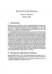
Figure 1:

The graph of ln(||F (X)||) for Example 4.1 with x(0) = 1

and Newton-HAM (NHAM) are reported. We utilize MATLAB 8. In Tables and Figures, the number of iterations (NI), the Euclidean norm of residual of government equation and CPU time, are presented. Example 4.1. Consider the following equation: f (x) = xex − 1 = 0,

(26)

The function f has at least one zero between 0 and 1. For x(0) = 1, the numerical results are shown in Table 1. For this initial point all methods are convergent, but the Newton method is apparently faster than other methods. For x(0) = 10, the numerical results are shown in Table 2. In this case, HM method is divergent, Newton method is faster than NHAM and HAM and results are more accurate than others. The number of iterations for NHAM is less than the others. For x(0) = −400, the numerical results are shown in the Table 3. In this example NHAM method is convergent and other methods are divergent.

66



NI 6 16 31 −

Numerical results for Example 4.1 with x(0) = 10 ||F (x(m) )|| CPU time result 2.160101e − 010 3.148814e + 000 Convergent 5.107026e − 014 2.622956e − 001 Convergent 3.594237e − 008 2.876829e + 000 Convergent 5.790573e + 003 4.081270e − 001 Divergent


10 5

log||F(XN)||

0 −5 −10 −15 −20 −25 −30 −35

0

5

Figure 2:

15 20 Number of Iteration

25

30

35

The graph of ln(||F (X)||) for Example 4.1 with x(0) = 10


10

NI 212 3 100 −

Numerical results for Example 4.1 with x(0) = −400

||F (x(m) )|| 2.403109e − 007 N an Inf inity N an

CPU time 6.452634e + 000 − − −

result Convergent Divergent Divergent Divergent


67

250 NHAM NEWTON HM

200

log||F(XN)||

150

100

50

0

−50

−100

0

Figure 3:

50


250

The graph of ln(||F (X)||) for Example 4.1 with x(0) = −400


200

NI 6 1 8 −

Numerical results for Example 4.2

||F (x(m) )|| 2.085579e − 008 N aN 2.247981e − 010 1.967763e + 009

CPU time 2.116125e + 000 − 3.105904e + 000 7.584255e − 001

Example 4.2. Consider following equations:  f1 (x, y, z, d) = xyz + d − 31 = 0,    f2 (x, y, z, d) = x + y + z + d − 11 = 0, f3 (x, y, z, d) = 2x + 3y + 4z + d − 35 = 0,    f4 (x, y, z, d) = x + z − y + d − 1 = 0,

result Convergent Divergent Convergent Divergent

(27)

[ ]T where F = f1 f2 f3 f4 . 11 −9 We know Xˆ1 = (2, 3, 5, 1) and Xˆ2 = ( 29 5 , 10 , 5, 10 ) are two solutions of F (X) = 0. For X (0) = (1, 1, 1, 1) , numerical results are shown in Table 4.

Newton Method is divergent because det(DF (X (0) )) = 0. But HAM and NHAM methods converge, and NHAM is faster than HAM. Example 4.3. Consider the following equations:

68

J. Izadian, R. Abrishami and M. Jalili 25 NHAM NEWTON HAM HM

20

15

10

log||F(XN)||

5

0

−5

−10

−15

−20

−25

1

Figure 4:

2

3

NI 8 101 18 −

6

7

8

The graph of ln(||F (X)||) for Example 4.2




||F (x(m) )|| 6.567317e − 010 5.030214e + 003 5.830347e − 008 5.242329e + 002

CPU time 8.196840e + 001 6.042236e + 000 3.106638e + 003 2.483993e + 000

result Convergent Divergent Convergent Divergent

 f1 (x1 , x2 , · · · , xn ) = (3 − 12 x1 )x1 − 2x2 + 1 = 0 ,      fi (x1 , x2 , · · · , xn ) = (3 − 12 xi )xi − xi−1 − 2xi+1 + 1 = 0 , 1 < i < n ,      fn (x1 , x2 , · · · , xn ) = (3 − 12 xn )xn − 2xn−1 + 1 = 0, (28) [ ]T that F = f1 f2 · · · fn . For n = 50 and X (0) = (100, 100, · · · , 100), numerical results are shown in Table 5. In this example HAM and NHAM are convergent to the exact solution ˆ = (1, ..., 1), but Newton method is divergent. Also NHAM is faster than X HAM. Results are shown in Figure 5. Example 4.4. Consider the following equations:   fk (x1 , x2 , · · · , xn ) = 10000xk xk+1 − 1 = 0, mod(k, 2) = 1, 

fk (x1 , x2 , · · · , xn ) = exp(−xk−1 ) + exp(−xk ) − 1.0001 = 0, mod(k, 2) = 0, (29)


69


15

10

log||F(XN)||

5

0

−5

−10

−15

−20

−25

0

10

20

Figure 5:

30

50 60 70 Number of Iteration

80

90

100

110

120



40

NI 13 12 23 −


||F (x(m) )|| 1.059758e − 009 1.112530e − 010 2.728830e + 056 4.211734e − 001

CPU time 5.152483e + 001 1.972995e + 001 1.128194e + 002 1.092275e + 002

result Convergent Convergent Divergent Convergent

[ ]T that F = f1 f2 · · · fn . For n = 100 and X (0) = (1, 0, 1, 0, 1, 0, 1, · · · , 0), numerical results are shown in Table 6. In this example Newton method, NHAM and HM are convergent, but HAM is divergent. Results are shown in Figure 6. Example 4.5. Consider the following equations:   f1 (x1 , x2 ) = exp(x1 ) + x1 x2 − 1 = 0, 

(30) f2 (x1 , x2 ) = sin(x1 x2 ) + x1 + x2 − 1 = 0,

[ ]T that F = f1 f2 · · · fn . For n = 100 and X (0) = (1, 0, 1, 0, 1, 0, 1, · · · , 0), numerical results are shown in Table 7. In this example all the methods are convergent. Results are shown in Figure 7.

70



120 100

log||F(XN)||

80 60 40 20 0 −20 −40

1 2 3 4 5 6 7 8 9 10 11 12 13 14 15 16 17 18 19 20 21 22 23 24 25 Number of Iteration

Figure 6:



NI 4 4 4 −


||F (x(m) )|| 1.993082e − 010 1.405720e − 012 1.187309e − 008 5.368713e − 006

CPU time 1.848117e + 000 2.472726e − 001 1.719704e + 000 1.380355e + 000

result Convergent Convergent Convergent Convergent


−5

log||F(XN)||

−10 −15 −20 −25 −30

1

Figure 7:


4



71

5 Conclusion In this paper, Newton-HAM (NHAM) applying control parameter h are proposed for solving systems of nonlinear equations. The results for all examples are convergent and also NHAM is faster than Homotopy method. The results demonstrate that by choosing a suitable h, HAM and NHAM methods are convergent. The numerical results show in general that the proposed method is effective and efficient and provides highly accurate results in a less number of iterations as compared by other methods. The main advantage of NHAM is the relative freedom of choosing initial guess. The appropriate proof convergence of NHAM can be continuation of the present work.

Acknowledgments The authors would like to thank the anonymous referees for valuable comments and also express appreciation for their constructive suggestions.

References 1. Abbasbandy, S. Improving Newton-Raphson method for nonlinear equations bymodifiedAdomian decompositionmethod, Applied Mathematics and Computation, 145 (2-3) (2003) 887-893. 2. Abbasbandy, S. and Jalili, M. Determination of optimal convergencecontrol parameter value in homotopy analysis method, Numerical Algorithms 64 (4) (2013) 593-605. 3. Abbasbandy, S., Tan, Y. and Liao, S.J. Newton-homotopy analysis method for nonlinear equations, Appl. Math. Comput. 188 (2007) 1794-1800. 4. Awawdeh, F. On new iterative method for solving systems of nonlinear equations, Numerical Algorithms, 54 (3) (2010) 395-409. 5. Babolian, E. and Jalili, M. Application of the Homotopy− Pad´ e technique in the prediction of optimal convergence-control paramete, Computational and Applied Mathematics, article in press. DOI:10.1007/s40314-014-01231, (2014). 6. Faires, J. and Burden, R. Numerical methods, Brooks Cole 3 edition, 2002. 7. Fang, L. and He, G. Some modifications of Newton’s method with higher order convergence for solving nonlinear equations, J. Comput. Appl. Math. 228 (2009) 296-303.

72


8. Fang, L. and He, G. An efficient Newton-type method with fifth-order convergence for Solving Nonlinear Equations, Comput. App. Math., 27(3) (2008) 269-274. 9. Izadian, J., Mohammadzade Attar, M. and Jalili, M. Numerical solution of deformation equations in Homotopy analysis method, Applied Mathematical Sciences, 6(8) (2012) 357-367. 10. Liao, S. On the homotopy analysis method for nonlinear problems, Applied Mathematics and Computation 147 (2004) 499-513. 11. Liao, S. Notes on the homotopy analysis method: Some definitions and theorems, Commun. Nonlinear Sci. Numer. Simulat., 14 (2009) 983-997. 12. Liao, S. The proposed Homotopy analysis technique for the solution of nonlinear problems, PhD thesis, Shanghai Jiao Tong University, 1992. 13. Liao, S. and Tan, Y. A general approach to obtain series solutions of nonlinear differential equations, Stud. Appl. Math 119 (2007) 297-354. 14. Liao, S. Beyond perturbation (Introduction to the homotopy analysis method), CHAPMAN and HALL , 2004. 15. Ku, C.Y., Yeih, W. and Liu, C.S. Solving nonlinear algebraic equations by a scalar Newton-homotopy continuation method, International Journal of Nonlinear Sciences and Numerical Simulation, 11(6) (2010) 435-450. 16. Stoer, J. and Bulrish, R. Introduction to numerical analysis, Springer, 1991. 17. Wu, Y. and Cheung, K.F. Two-parameter homotopy method for nonlinear equations, Numerical Algorithms, 53(4) (2010) 555-572.

‫ﯾﮏ روش ﺟﺪﯾﺪ ﺑﺮای ﺣﻞ دﺳﺘﮕﺎه ﻣﻌﺎدﻻت ﻏﯿﺮ ﺧﻄﯽ ﺑﺎ اﺳﺘﻔﺎده از روش ﻧﯿﻮﺗﻦ و ‪HAM‬‬ ‫ﺟﻼل اﯾﺰدﯾﺎن ‪ ،۱‬ﻏﻼﻣﺮﺿﺎ اﺑﺮﯾﺸﻤﯽ ‪ ،۱‬و ﻣﺮﯾﻢ ﺟﻠﯿﻠﯽ‬

‫‪۲‬‬

‫‪۱‬داﻧﺸﮕﺎه آزاد ﺳﻼﻣﯽ‪ ،‬واﺣﺪ ﻣﺸﻬﺪ‪ ،‬داﻧﺸﮑﺪه ﻋﻠﻮم‪ ،‬ﮔﺮوه رﯾﺎﺿﯽ‬ ‫‪۲‬داﻧﺸﮕﺎه آزاد ﺳﻼﻣﯽ‪ ،‬واﺣﺪ ﻧﯿﺸﺎﺑﻮر‪ ،‬داﻧﺸﮑﺪه ﻋﻠﻮم‪ ،‬ﮔﺮوه رﯾﺎﺿﯽ‬

‫ﭼﮑﯿﺪه ‪:‬‬ ‫ﯾﮏ روش ﺟﺪﯾﺪ ﺑﺮای ﺣﻞ دﺳﺘﮕﺎه ﻣﻌﺎدﻻت ﻏﯿﺮ ﺧﻄﯽ ﺑﺎ اﺳﺘﻔﺎده از روش ﻧﯿﻮﺗﻦ و روش آﻧﺎﻟﯿﺰ ﻫﻤﻮﺗﻮﭘﯽ‬ ‫)‪ (HAM‬اراﺋﻪ ﻣﯽ ﺷﻮد‪ .‬اﻓﺰاﯾﺶ ﺳﺮﻋﺖ ﻧﺮخ ﻫﻤﮕﺮاﯾﯽ ‪ HAM‬و ﺑﺪﺳﺖ آوردن ﺳﺮﻋﺖ درﺟﻪ دوم ﻫﻤﮕﺮاﯾﯽ‬ ‫ﮐﻠﯽ اﻫﺪاف اﺻﻠﯽ اﯾﻦ روش اﺳﺖ‪ .‬ﻧﺘﺎﯾﺞ ﻋﺪدی ﮐﺎراﯾﯽ و ﻋﻤﻠﮑﺮد روش ﭘﯿﺸﻨﻬﺎدی را در ﻣﻘﺎﯾﺴﻪ ﺑﺎ روش‬ ‫ﻫﻤﻮﺗﻮﭘﯽ ﻣﻌﻤﻮﻟﯽ‪ ،‬روش ﻧﯿﻮﺗﻦ و ‪ HAM‬ﻧﺸﺎن ﻣﯽ دﻫﺪ‪ ،‬ﮐﻪ در اﯾﻦ روش آزادی ﺑﺴﯿﺎری در اﻧﺘﺨﺎب ﺣﺪس‬ ‫اوﻟﯿﻪ دارﯾﻢ‪.‬‬ ‫ﮐﻠﻤﺎت ﮐﻠﯿﺪی ‪ :‬روش آﻧﺎﻟﯿﺰ ﻫﻤﻮﺗﻮﭘﯽ؛ ﻣﻌﺎدﻻت دﮔﺮدﯾﺴﯽ ﻣﺮﺗﺒﻪ ﺻﻔﺮ؛ ﭘﺎراﻣﺘﺮ ﮐﻨﺘﺮل ﻫﻤﮕﺮاﯾﯽ؛ روش‬ ‫ﻧﯿﻮﺗﻦ؛ روش ﺗﮑﺮاری؛ روش ﺗﮑﺮاری ﭼﻨﺪ ﮔﺎم؛ ﻣﺮﺗﺒﻪ ﻫﻤﮕﺮاﯾﯽ‪.‬‬