SOLVING A SYSTEM OF NONLINEAR EQUATIONS WITH THE USE ...

Journal of Applied Mathematics and Computational Mechanics 2016, 15(2), 53-64 www.amcm.pcz.pl p-ISSN 2299-9965 DOI: 10.17512/jamcm.2016.2.06 e-ISSN 2353-0588

SOLVING A SYSTEM OF NONLINEAR EQUATIONS WITH THE USE OF OPTIMIZATION METHODS IN PROBLEMS RELATED TO THE WHEEL-RAIL CONTACT

Mariola Jureczko, Sławomir Duda Institute of Theoretical and Applied Mechanics, Silesian University of Technology Gliwice, Poland [email protected], [email protected]

Abstract. The article presents the methods for defining the geometry of the contact surface between a rigid wheel and a rigid rail. The calculation model that has been developed allowed for any arrangement of the wheel in relation to the rail. This allowed for the creation of a system of nonlinear equations, the solution of which allows one to determine the presumable wheel-rail contact points. The search for the solution of the system of strongly nonlinear equations was conducted using a few optimization methods. This allowed one to study both the selection of the starting point and the convergence of the method. Keywords: wheel-rail contact, system of nonlinear equations, Newton’s method, trust region method, Levenberg-Marquardt method, damped Newton’s method

1. Introduction Systems of nonlinear equations occur in mathematical models of physical phenomena in various fields of science such as mechanics, engineering, medicine, chemistry or robotics. Their proper solution at a low computational cost is significant in the case of studying model physical systems in which the solution of nonlinear equations is one of the stages in solving a more complex problem and where the precision of the solution has an effect on the solution of the entire model. Among others, this concerns the numerical simulations of a rail-vehicle movement on any track. The dynamic equations describing the complex system of a vehicle, drive and track are most often highly complex and require considerable amounts of time for calculation. This substantiates the need to find an effective tool that would serve as the solution of individual models. One of the methods to solve the problem of the wheel-rail interaction is to define the geometries of the contacting surfaces as parameters. Finding the contact point between the cooperating elements - the wheel and the rail - is conducted by solving a system of four nonlinear algebraic equations.

54

M. Jureczko, S. Duda

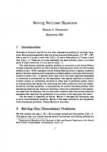
The application of iterative methods for solving the problem referred to above requires the starting point to be provided - that is, the precise indication of a contact point. Otherwise the method shall not be convergent. This especially concerns the analyses of cases where the continuity of contact between the wheel and the rail is interrupted (e.g. wheel motion at the railway junction - Fig. 1). The solution of such a problem involves the determination of all possible solutions. It is thus a specific problem of multicriteria optimization.

axis y [m]

contact point between rail and tread of the wheel

candidate to contact point between rail and flange of the wheel axis x [m]

Fig. 1. Wheel motion at the railway junction with possibility of two-point contact

There are many optimization and numerical methods for solving systems of equations. These, however, mostly concern finding solutions for single linear or nonlinear equations, systems of linear equation with one or many unknowns, or systems of nonlinear equations with just one unknown. In the case of systems of equations that do not exhibit the properties of polynomials of linear functions and have many variables, however, there are no means which guarantee the determination of all possible solutions [1-3]. One of the applications of optimization methods is the determination of radixes of nonlinear equations or systems of nonlinear equations. There are many methods to obtain approximate solutions for nonlinear equations with one variable. Iterative methods are used most commonly, for example the bisection method, the secant method, the false-position method, Brent’s method or Simple Fixed - Point Iteration. One should remember, however, that using the methods referred to above, the roots of the equation are determined with a precision [4-6]. Wishing to determine all possible solutions of a system of nonlinear equations may be presented as:  f1 ( x1 ,..., xi ,..., xn ) = 0  ⋮    f i ( x1 ,..., xi ,..., xn ) = 0  ⋮   f n ( x1 ,..., xi ,..., xn ) = 0

(1)

Solving a system of nonlinear equations with the use of optimization methods in problems related …

55

where n stands for the size of the problem, xi refers to the i-th independent variable, and fi(.) is the i-th nonlinear equation, one should modify the methods presented above or develop a hybrid method. The problem in solving the system (1) may be transformed to the form of an optimization problem consisting in the determination of the optimum of the objective function expressed as: min xF

n

(x ) = ∑ f i (x1 ,..., xi ,..., xn ) .

(2)

i =1

It is evident that after such a transformation, the determined global minimum of the equation (2) is substituted for the (1). As a result, the application of the optimization method in the solution of equation (2) shall allow one to determine solution of the problem presented in the following form (1).

2. The application of optimization methods in solving a system of nonlinear equations with multiple variables Let us assume that F = [f1, f2,…, fn]T is a n-dimensional vector corresponding to the set of the function, while x = [x1, x2,…, xn]T denotes a n-dimensional vector of independent variables. 2.1. Newton’s method To solve the problem of the system of a n-number of nonlinear equations represented by the dependence (1), the basic Newton’s method is generalized to a n-number of dimensions [5, 7-9]. Assuming that the x k vector is a certain approximation of the searched solution and omitting the terms of higher order in the expansion of individual functions of many variables into Taylor’s series, that are subsequently equated to zero, one will obtain an approximate dependence for the k + 1 of the iteration:

( )(

)

( )

J x k ⋅ x k +1 − x k = −F x k .

(3)

The J(xk) matrix of partial derivatives is the Jacobian matrix. The solution of the equation (3) in relation to the x k +1 vector equals:

( ) ( )

x k +1 = x k − J −1 x k ⋅ F x k .

(4)

The termination criterion in Newton’s method assumes the following form: x k +1 − x k ≤ ε ,

(5)

where ε denotes the required precision of calculations and ||.|| is the Euclidean norm of the vector.

56

M. Jureczko, S. Duda

2.2. Damped Newton’s method One of the methods used to mitigate the problem of the lack of convergence of Newton’s method, or, to be more precise, its dependence on the selection of the starting point, is the combination of the idea of minimization with Newton’s method. What emerges is the hybrid method. With each iteration of the classic Newton’s method, after determining the direction of research, the method adds a minimization of the λ length of that step in such a way that the Euclidean norm of the F vector value in the subsequent approximation of the starting point is decreased along with the progress of the optimization process. This modified Newton’s method is called the damped Newton’s method. In that method, subsequent approximations of the stationary point are determined using the dependence [10]: x k +1 = x k + λ ⋅ ( − J −1 (x k ) ⋅ F (x k )) ,

(6)

where the λ step length is selected in such a way as to ensure that the following condition is fulfilled:

( ) (

)

( ) ( ).

− J −1 x k ⋅ F xk +1 < −J −1 xk ⋅ F x k

(7)

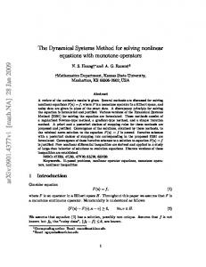
This way, the direction of the step in the damped Newton’s method is a local direction of decrease in the value of the F function vector. A shift by the complete length of Newton’s step determined in this way, however, does not need to lead to a decrease in the F value. This is why the length of the step determined in such a way is usually decreased by half. Instead of using a half-step, however, another strategy of finding the λ, which also leads to the decrease in the F value, may be applied. If the λ value drops beneath a certain acceptable threshold, the calculations should be stopped, but the dependence (7) guarantees that such a λ exists, where λ ⋅ ( − J −1 (x k ) ⋅ F(x k )) leads to a decrease in the value of the F vector. START

The choice: x0, λ=1 Calculation of dk xpom = xk + λdk λ = λ/2 F(xpom) < F(xk)

NO

YES

xk+1 = xpom FINISH

Fig. 2. Block diagram representing the algorithm of the damped Newton’s method

Solving a system of nonlinear equations with the use of optimization methods in problems related …

57

Figure 2 shows a block diagram representing the algorithm of the damped Newton’s method. 2.3. Levenberg-Marquardt method Another algorithm that is often applied for solving systems of nonlinear equations is the Levenberg-Marquardt method (abbreviated as LM) [11, 12]. In the case of this method, in the beginning of the algorithm the method of steepest descent is applied for subsequent approximations of the stationary point relatively distant from the minimum of the F vector. In this method, the direction of search providing the steepest descent of the function value is determined based on the values of the sensitivity coefficients of the function in relation to its individual parameters and based on the calculation results from the previous step. Subsequently, near the minimum of the F vector, the method of steepest descent is replaced with the method of linearization of the regression function such as the Gauss-Newton’s method. Subsequently, the search for the minimum is preceded by an analytical determination of its location in such a way as if the problem was linear. Further possible iterations are used for a precise localization of the minimum. This may be necessary due to a deviation related to the simplification to a linear problem. In the LM method, subsequent approximations of the stationary point are determined using the dependence:

(

x k +1 = x k − H k + λ ⋅ diag  H k 

)

−1

( )

⋅ ∇F x k

(8)

where: Hk - hessian of the F(x) function vector in the xk point, λ - regulation parameter, k diag[H ] - diagonal matrix of the hessian of the F(x) function vector in the xk point, ∇F (x k ) - gradient of the F(x) function vector in the xk point. Generally, the sequence of the LM method may be presented as follows: 1. Assume a starting point. 2. Determine the value of the next approximation of the stationary point in line with the equation (8). 3. Calculate the value of deviation in the xk+1 point. 4. If the deviation has increased, return to the xk value, increase the value of λ by k orders of magnitude and return to step 2 (the linear approximation of the minimized function in the neighborhood of xk turned out to be insufficiently accurate, so the „impact” of the steepest descent method is increased). 5. If the deviation has decreased, accept the step and decrease the value of λ by k orders of magnitude (the assumption of linearity of the minimized function in the neighborhood of xk turned out to be insufficiently accurate, so the “impact” of the Gauss-Newton’s method is increased).

58

M. Jureczko, S. Duda

2.4. Trust region method Trust region methods (abbreviated as TR) are relatively new optimization algorithms [13, 14]. These methods are based upon a notion that an algorithm exhibits a priori knowledge regarding the local behaviour of the objective function and that this knowledge is “extended” to much wider regions. The region in which the objective function is approximated is called the trust region. The trust region is most often assumed to be a sphere with an rk radius. In each iteration the trust area concentrated around the best xk solution is determined. Subsequently, the FM(x) function is determined, which approximates the primary objective function to a certain extent. This way, the complicated optimization problem is down to solving a quadratic programming problem, that is, the determination of the xMk point minimizing the FM(x) function. It is known that the solution obtained in such a way will differ from the actual minimum of the F function within the trust region, but it is assumed that the difference will not be significant. Another significant assumption is the assumption that the inequality:

( ) ( )

F x Mk < F x k −1

(9)

will be satisfied in each iteration step. It meaning that the value of the F function shall decrease with each iteration. The length of the step in the trust region method is usually determined before the correction of the direction. If the decrease in the value of the FM(x) function is achieved, the assumed trust region is assumed to be correct. If, on the other hand, the improvement is too subtle or no improvement is noted, the trust region should be changed. This means that the rk radius of the trust region should be properly adjusted to the variability of the F function. The general sequence of TR method is as follows: 1. Initialization: Select an x0 starting point. Determine the initial rk trust region. 2. For the xk point, determine the model of FM(x) function in its neighbourhood. 3. Find such an ~ x k approximation of point that: x Mk = arg

min F x∈Ω (x k ) M

(x ) k

(10)

4. Verify whether the size of the trust region had been selected properly. If so, k substitute x = ~ x k and continue to step 6. Otherwise continue with step 5. 5. Decrease the trust region to rs, substitute rk:= rs and go to step 3. 6. If the termination criterion is fulfilled, the xk should be assumed to be the optimal solution. Otherwise, go to step 7. 7. Verify whether the trust region should be increased to rB. If so, substitute rk: = rB, and continue to step 8. Otherwise go to step 1. 8. Substitute k := k + 1, go to step 2.

Solving a system of nonlinear equations with the use of optimization methods in problems related …

59

3. Formulating a system of nonlinear equations The surface area of a wheel or rail was obtained by drawing flat curves constituting the profile of the wheel or rail around the rotation axis of the wheel or along the line of the track. The definition of the geometries of contact surfaces between the rigid wheel and the rigid rail is based on four independent parameters: sr and ur describing the geometry of the rail surfaces and sw and uw describing the surface of the wheel - as presented in Figure 3.

Fig. 3. Wheel and rail surface parameters

The location of the radius of the vector in the Q contact point in a system of coordinates related to the wheel or the rail is only a function of the parameters of their surfaces. Considering the areas of the rail and the wheel determined by the p(sr,ur) and q(sw,uw), parametric functions, the surface of the wheel will remain in contact with the surface of the rail when [15]: • normal vectors to the nr and nw surfaces of the presumed contact points must be in parallel. This condition means that the nr vector exhibits a zero projection on the tsw and tuw tangent vector:

nT t s = 0 n r × n w = 0 ≡  Tr uw n r t w = 0

(11)

• the d vector representing the distance between the presumed contact points must

be in parallel to the n w. This condition may be mathematically presented as:

dT t s = 0 d × n w = 0 ≡  T uw d t w = 0

(12)

60

M. Jureczko, S. Duda

The geometric conditions presented in equations (11) and (12) are four nonlinear equations with four unknowns. The system of equations provides a solution in the form of locations of the presumable contact points. The presented formula used for finding the presumed contact points is limited to parametric convex surfaces. In reality, if one or both of the surfaces were concave, the formula could lead to multiple solutions.

4. Formulating the optimization problem To conduct the analysis of the impact of the applied optimization method on the determination of the contact point between the surfaces of the rail and wheel, a calculation model has been developed for the wheel-rail system. The model has been presented in Figure 4. By applying various values of the ϕ angle - rotation about longitudinal axis (roll, sway), the model allows for any orientation of the wheel in relation to the rail.

Fig. 4. The cooperation model of wheels with rail

The parameters defining the geometry of the wheel-rail contact surface have been selected in the optimization process as decision variables. The parameters were as follows: sr - length of the space curve of the rail, that is, the distance of the rail profile at which the contact point is located from the point in which the analysis has been started [m], ur - a coordinate specifying the lateral position of the contact point in the system of coordinates of the rail profile [m], sw - value of the rotation angle of the system of coordinates of the wheel profile in relation to the system of coordinates related to the finite element node, that is, specifying the angular displacement of the contact point [rad], uw - a coordinate specifying the lateral position of the contact point in the system of coordinates of the wheel profile [m]. The solution of the optimization problem presented in that way consisted in the determination of roots of the system of strongly nonlinear equations.

61

Solving a system of nonlinear equations with the use of optimization methods in problems related …

An additional hindrance in the development of a useful algorithm was constituted by the fact that the wheel could be positioned under various angles in relation to the rail. This is why the calculations were conducted for various ϕ angles of superelevation, which means that the conditions assumed in [16, 17] allowed one to formulate a system of nonlinear equations that may not contain satisfying solutions. Limitations resulting from the assumed model of the wheel-rail contact geometry model were superimposed on each of the decision variables. The form was as follows:

−1 ≤ sr ≤ 1

(13)

− 0.039 ≤ ur ≤ 0.039

(14)

− 0.7854 ≤ sw ≤ 0.7854

(15)

− 0.03 ≤ uw ≤ 0.03 (16) The optimization calculations have been conducted using the methods described in Section 2. a)

b)

c)

d)

Fig. 5. Diagram presenting the values of each of the variables depending on the superelevation angle: a) x1 variable, b) x2 variable, c) x3 variable, d) x4 variable, for x = [1;0;0;0]

62

M. Jureczko, S. Duda

a)

b)

c)

d)

Fig. 6. Diagram presenting the values of each of the variables depending on the superelevation angle: a) x1 variable, b) x2 variable, c) x3 variable, d) x4 variable, for x = [0.1;‒0.0062;0;0.0031]

One of the greatest limitations related to the application of iterative algorithms is the lack of possibility to obtain all possible solutions. The achieved result is dependent on the selection of the starting point for calculations. This is why the calculations were conducted for several starting points that have been selected based on the authors’ experience. The selected starting points were as follows: x = [1;0;0;0] and x = [0.1;‒0.0062;0;0.0031]. Figures 5 and 6 present the optimal values of each of the parameters obtained using each of the optimization methods, depending on the superelevation angle in the selection of the starting point in [1;0;0;0] (Fig. 5) and [0.1;‒0.0062;0;0.0031] (Fig. 6).

7. Conclusions One of the methods to detect a failure of a given optimization method is to verify the number of conducted iterations. If that number exceeds a given limit, the optimization process is stopped. In case of the applied optimization methods, the analysis of their course allows one to confirm the validity of their selection.

Solving a system of nonlinear equations with the use of optimization methods in problems related …

63

While analysing the results obtained for the superelevation angle of 0° and 5°, one may note that all the analyzed methods exhibited convergence to the optimal solution, while TR appeared to be the fastest of the methods. The DN and LM methods (for the 0° angle), on the other hand, were the most time-consuming. The DN method has been the most independent from the selection of the starting point. In case of calculations for the superelevation angle of 10°, the TR method was the quickest and the Newton’s method appeared to be the most timeconsuming and the least independent from the selection of the starting point. In case of the superelevation angle in the 15°÷30° range, only the LM and TR methods exhibited convergence to the stationary point. The obtained values of the starting point, however, were different. Changes of the trust field radius in the TR method did not improve the result. While analyzing the time of computation, the trust field method appeared to be the most efficient one. In case of the superelevation angle in the 35°÷45° range, all methods exhibited convergence to a solution which was not the root of the analyzed system of equations. Thus, the minimum that was determined was local. The obtained results have confirmed the prior conclusion of the authors, that is, the impact of the selection of the starting point on the obtained result. Thus, the selection of top or bottom limits imposed on each of the decision variables as the starting points - which was not presented in this article - did not allow one to determine the solutions from the field of possible solutions. Table 1 presents the best results obtained for each of the superelevation angles. The TR and LM were the methods that were the most independent from the selection of the starting point. Table 1 The best results obtained for each of the superelevation angles Superelevation angle [°]

xˆ [m]

F(xˆ )

Methods

0°

[0.1; –0.0061; 0; 0.0032]

10–6·[0; 0.1346; 0; 0.0042]

all

5°

[0.1; –0.0085; 0; 0.0002]

10

–12

·[0; 0.1168; 0; 0.0023]

[0.1; –0.0214; 0; –0.0204]

15°

[0.1; –0.0218; 0; –0.0232]

10–16·[0; -0.8327; 0; 0.4857]

LM

20°

[0.1; –0.0199; 0; –0.0144]

10–10·[0; 0.9305; 0; –0.0167]

LM, TR

[0.1; –0.0129; 0; –0.0049]

10

·[0; –0.8047; 0; –0.2130]

all

10°

25°

10

–10

–12

all

·[0; 0.1113; 0; 0.1106]

LM, TR

–9

30°

[0.1; –0.0220; 0; –0.0245]

10 ·[0; 0.8506; 0; 0.0782]

LM, TR

35°

[0.1; –0.0236; 0; –0.03]

[0; –0.0087; 0; 0.0120]

LM, TR

40°

[0.1; –0.0259; 0; –0.03]

[0; –0.0418; 0; 0.0522]

LM, TR

45°

[0.1; –0.0285; 0; –0.03]

[0; –0.1011; 0; 0.0840]

LM, TR

While analysing the methods of determining four nonlinear equations with four unknowns (as described in Section 3), one may note that they are limited to finding

64

M. Jureczko, S. Duda

only the presumable points of contact of parametric convex surfaces. One may presume that in case of a greater superelevation angle, one of the surfaces would be concave. Then, in the case of such assumed geometric limitations (see the limitations superimposed on each of the decision variables), it may not allow one to determine the roots. Acknowledgement This paper was realized within the framework of BK-217/RMT3/2015.

References [1] [2] [3] [4] [5] [6] [7] [8] [9] [10]

[11] [12]

[13]

[14] [15] [16] [17]

Grosan C., Abraham A., A new approach for solving nonlinear equations systems, IEEE Transactions on Systems, Man, and Cybernetics - part A: Systems and Humans 2008, 38, 3, 698-714. Nedzhibov G.H., A family of multi-point iterative methods for solving systems of nonlinear equations, Comput. Appl. Math. 2008, 222, 244-250. Taheri S., Mammadov M., Solving systems of nonlinear equations using a globally convergent optimization algorithm, Global J. of Tech. and Optim. 2012, 3, 132-138. Chapra S.C., Canale R.P., Numerical Methods for Engineers, 6th edition, McGraw-Hill Companies, 2010. Yang Y.W., Cao W., Chung T., Morris J., Applied Numerical Methods Using Matlab®, John Wiley & Sons, 2005. Kiusalaas J., Numerical Methods in Engineering with Matlab®, Cambridge University Press, 2009. Jureczko M., Metody optymalizacji - przykłady zadań z rozwiązaniami i komentarzami, Wydawnictwo Pracowni Komputerowej Jacka Skalmierskiego, Gliwice 2009. Quarteroni A., Saleri F., Scientific Computing with Matlab and Octave, 2nd edition, Springer, 2006. Mathews J.H., Fink K.D., Numerical Methods Using Matlab, Prentice Hall, 1999. Deuflhard P., A modified Newton method for the solution of ill-conditioned systems of nonlinear equations with application to multiple shooting, Numerical Mathematics No 22, Springer Verlag, 1974, 289-315. Hagan M.T., Menhaj M.B., Training feedforward networks with the Marquardt algorithm, IEEE Trans. on Neural Networks 1994, 5, 6, 989-993. Transtrum M.K., Sethna J.P., Improvements to the Levenberg-Marquardt algorithm for nonlinear least-squares minimization, Preprint submitted to Journal of Computational Physics, January 30, 2012. Yuan Y.X., A review of trust region algorithms for optimization, ICM99: Proc. 4th Int. Congress on Industrial and Applied Mathematics, eds. J.M. Ball, J.C.R. Hunt, Oxford University Press 2000, 271-282. Yuan Y.X., Recent advances in trust region algorithms, Math. Program., Ser. B 2015, 249-281. Mortenson M.E., Geometric Modeling, Wiley, New York 1985. Duda S., Modelowanie i symulacja numeryczna zjawisk dynamicznych w elektrycznych pojazdach szynowych. Monografia nr 405, Wydawnictwo Politechniki Śląskiej, Gliwice 2012. Duda S., Numerical simulations of the wheel-rail traction forces using the electromechanical model of an electric locomotive, J. Theor. Appl. Mech. 2014, 52, 2, 395-404.