To incorporate numeric values, some extensions of the COBWEB system are proposed, such as .... The process of model formation is the same as a model-based clustering, since the .... It is natural to have a hierarchical order between the model-based formal ..... model g2 whose member data are the instances of C4.
A model-based conceptual clustering of moving objects in video surveillance Jeongkyu Lee∗ , Pragya Rajauria∗ , Subodh Kumar Shah∗ Department of Computer Sciences & Engineering University of Bridgeport Bridgeport, CT 06604-5692 U.S.A. ABSTRACT Data mining techniques have been applied in video databases to identify various patterns or groups. Clustering analysis is used to find the patterns and groups of moving objects in video surveillance systems. Most existing methods for the clustering focus on finding the optimum of overall partitioning. However, these approaches cannot provide meaningful descriptions of the clusters. Also, they are not very suitable for moving object databases since video data have spatial and temporal characteristics, and high-dimensional attributes. In this paper, we propose a model-based conceptual clustering (MCC) of moving objects in video surveillance based on a formal concept analysis. Our proposed MCC consists of three steps: ‘model formation’, ‘model-based concept analysis’, and ‘concept graph generation’. The generated concept graph provides conceptual descriptions of moving objects. In order to assess the proposed approach, we conduct comprehensive experiments with artificial and real video surveillance data sets. The experimental results indicate that our MCC dominates two other methods, i.e., generality-based and error-based conceptual clustering algorithms, in terms of quality of concepts. Keywords: Conceptual clustering, formal concept analysis, EM, moving objects
1. INTRODUCTION The use of data mining techniques in many applications has increased enormously with the recent advances in computer power. Much of data collected in diverse areas of the industrial and scientific world contains valuable knowledge that is not easily retrievable. The knowledge identified by data mining may take form of predictive rules, clusters, patterns, and conceptual descriptions. To take this advantage into video content analysis, several studies have proposed the video data mining.1–4 Clustering analysis, or simply clustering, is one of popular data mining techniques used to find the patterns and groups in video data.3, 4 Most existing methods for the clustering focus on finding the optimum of overall partitioning. However, these approaches cannot provide any descriptions of the clusters. Conceptual clustering not only partitions the data, but generates resulting clusters that can be summarized by a conceptual description. For example, COBWEB5 is an incremental clustering algorithm based on probabilistic categorization trees. However, pure COBWEB only supports nominal attributes. In other words, it cannot be used for abstracting numeric data. To incorporate numeric values, some extensions of the COBWEB system are proposed, such as COBWEB/3,6 ECOBWEB,7 AUTOCLASS,8 Generality-based conceptual clustering (GCC),9 and Error-based conceptual clustering (ECC).10 However, all of the methods mentioned above do not represent the relations among the clusters or the appropriate meaning of each cluster. Also, they are not very suitable for moving object databases since video data have spatial and temporal characteristics, and high-dimensional attributes. To address these, we propose a model-based conceptual clustering algorithm (MCC) of moving objects in video surveillance systems. The proposed MCC differs from existing methods as follows: (1) it utilizes a formal concept analysis to generate concepts, (2) it uses models instead of individual data objects to handle complicated moving objects, and (3) it provides conceptual descriptions of moving object databases such as significant features and relationships. The rest of the paper is organized as follows. In Section 2, we present a model-based conceptual clustering algorithm of moving objects in video surveillance systems. The performance study is reported in Section 3. Finally, Section 4 presents some concluding remarks. ∗
E-mail: {jelee, prajauri, subodhs}@bridgeport.edu
2. MODEL-BASED CONCEPTUAL CLUSTERING In this section, we propose a model-based conceptual clustering (MCC) of moving objects, which is based on a formal concept analysis.11–14 Figure 1 shows the process of MCC of moving objects. As seen in the figure, MCC consists of three steps. Step 1 is a ‘model formation’. We form a set of models from moving object database by using a clustering analysis. Among existing clustering techniques, we choose Expectation Maximization (EM) algorithm since we can use the byproducts of EM, i.e., the extracted model parameters and the expectation values in the following steps. Each model, i.e., cluster, is characterized by a set of parameters used for computing significance values of features. Step 2 is a ‘model-based concept analysis’. In order to extract formal concepts from the models formed in Step 1, we propose a model-based formal concept analysis (MFCA) by applying the models to a formal concept analysis. Step 3 is a ‘concept graph generation’. This step refines the formal concepts and relations obtained in Step 2. MFCA typically produces a large number of concepts. There exist some number of similar concepts that need to be merged into a single concept. The final result of MCC is a concept graph that includes a set of conceptual nodes and relational edges. From the concept graph we can generate conceptual descriptions of moving object data.
Model-based Conceptual Clustering Step 1
Moving object database
Step 2
model formation
model-based concept analysis
Step 3
concept graph generation
Figure 1. The process of model-based conceptual clustering of moving objects
2.1. Model Formation In this subsection, we first introduce a distance function ST ED (Spatio-Temporal Edit Distance) that measures the dissimilarity between two moving objects. Then, we describe a model formation based on EM clustering with ST ED. 2.1.1. Spatio-Temporal Edit Distance In order to cluster moving objects, we need an appropriate distance function that can measure the dissimilarity s between two moving objects considering their spatial and temporal characteristic. Let M Om and M Ont be the th th s and the t moving objects with time m and n, respectively. s s M Om =< ~v1s , . . . , ~vm >,
M Ont =< ~v1t , . . . , ~vnt >
where ~vi is a feature vector of dimension d, which has the observed values of a moving object at time slot i. The s distance function ST ED between M Om and M Ont is defined as follows: s Definition 1. The spatio-temporal edit distance (STED) between two moving objects M Om and M Ont is: s s s ST ED(M Om , M Ont ) = min[ST ED(M Om−1 , M Ont ) + dst (~vm , ~g ), s t ST ED(M Om , M On−1 ) + dst (~g , ~vnt ), s t s ST ED(M Om−1 , M On−1 ) + dst (~vm , ~vnt )]
where ~g is an edited vector with ~gi =
~ vi−1 +~ vi , 2
and the cost function dst (~vis , ~vjt ) =
Pd l=1
t s |. − vj,l ωl |vi,l
Pd s In the cost function dst of Definition 1, ωl is a weight of the lth feature of M O where l=1 ωl = 1, and vi,l th s th indicates a value of the l component of ~vi . The weight of the l feature, ωl is selected based on the variance (σl ) of its feature as follows: log(1 − σl ) , ωl = Pd k=1 log(1 − σk )
(1 ≤ l ≤ d)
(1)
If a certain feature has a higher value of variance, it is considered as less important feature than others, i.e., a lower value of weight. 2.1.2. EM Clustering of Moving Objects The process of model formation is the same as a model-based clustering, since the clustering conducts unsupervised learning to find models of moving objects, which are characterized by a set of parameters. In order to find the models of moving objects, we employ a model-based EM clustering4, 15 with ST ED in Definition 1. Given M mutually independent sample M Os, Y = {y1 , . . . , yM }, the d-dimensional Gaussian mixture density with ST ED is given by K X 2 1 wk p(yj |Θ) = e− 2σ2 ST ED(yj ,µk ) (2) 1/2 2π |σk | k=1 where K is the number of models, and wk ( log-likelihood (L) of K mixture model is
PK k=1
L(Θ|Y) = log
M Y
wk = 1) is the membership probability of the k th model. The
p(yj |Θ) =
j=1
M X
log
j=1
K X
wk pk (yj |θk )
(3)
k=1
where each θk is the set of parameters of the k th model. In order to find appropriate models, we estimate the optimal values of the parameters (θk ) and the weights (wk ) in Equation (3) using EM algorithm, which is a common procedure used to find the Maximum Likelihood Estimates (MLE) of the parameters iteratively. The EM algorithm produces the MLE of the unknown parameters using two alternating steps: E-step: It evaluates the posterior probability of yj , belonging to each model k. Let hjk be the probability of the j th M O for a model k, then it can be defined as follows: hjk = P (k|yj , θk ) =
wk pk (yj |θk )
(4)
M-step: It computes the new parameter value that maximizes the probability using hjk in E-step as follows: M 1 X wk = hjk , M j=1
PM
PM µk =
j=1 hjk yj PM j=1 hjk
,
σk =
j=1
hjk ST ED(yj , µk )2 PM j=1 hjk
The iteration of E and M steps is stopped when wk is converged for all k. After the maximum likelihood ˆ in Equation (3) are decided, each M O is assigned to a model. model parameters (Θ) The benefits of model formation in the proposed conceptual clustering are as follows: (1) it simplifies the computation of a conceptual clustering algorithm since the number of objects is reduced to the number of models that represent their specific patterns, and (2) byproducts of the EM algorithm, i.e., the extracted model parameters (Θ) and the expectation (hjk ) play an important role in conceptual clustering since they provide the relationships between models and features.
2.2. Model-based Concept Analysis The second step of MCC is a model-based concept analysis to find formal concepts of modelled moving object data. Although the model formation in Step 1 provides a set of models where similar moving objects are grouped, it does not consider interpreting the obtained models. In other words, it is hard to understand what the meaning of each model is, and how the models are formed. In order to address these, we employ a formal concept analysis (FCA) that was introduced by Wille.11, 12 FCA has been used for data analysis and knowledge representation. We propose a model-based concept analysis (MFCA), which incorporates a model-based statistical data analysis with FCA to represent conceptual meaning of moving object data. The MFCA starts with a model-based formal context that is defined as: Definition 2. A model-based formal context is a triple K = (G, F, I), where • G is a set of models characterized by Θ, • F is a set of features, and • I is a set of relations between G and F (i.e. I ⊆ G × F ). Each relation (g, f ) ∈ I has a significance value λ(g, f ). In the model-based formal context, G consists of the models determined in Step 1 instead of all data objects. Each model is characterized by a set of parameters (Θ). A set of features (F ) consists of d number of observed features in M O. A set of relations I indicates how much each feature is relevant to each model. The relevance between the k th model gk and the lth feature fl is represented as the significance value λ(gk , fl ), which is computed by exploiting a feature selection technique in data mining.16 Let yF and yF −{fl } be the full feature vector, and the feature vector without the lth feature, respectively. Consider two posterior probabilities (Pi,k,F , Pi,k,F −{fl } ) of the k th model based on the full feature vector (yF ), and the feature vector without fl feature (yF −{fl } ) as follows. Pi,k,F = P (yi,F |θk,F ),
Pi,k,F −{fl } = P (yi,F −{fl } |θk,F −{fl } )
Pm Pm where i=1 Pi,k,F = 1 and i=1 Pi,k,F −{fl } = 1 with m number of objects in the k th model. If fl is a completely insignificant feature in the k th model, then Pi,k,F is equal to Pi,k,F −{fl } . Otherwise, the difference between two probabilities provides a significance value of fl in the model. In order to measure a difference between two probabilities, we use the Kullback-Leibler divergence (KLD).17 The significance value of the lth feature (fl ) in the k th cluster is defined as: ¯ m ¯ X ¯ ¯ ¯Pi,k,F log Pi,k,F ¯ λ(gk , fl ) = (5) ¯ Pi,k,F −{fl } ¯ i=1 The higher the value of λ, the more significance of the feature in a model. Then, we determine all relations between a set of models G and a set of features F . A model-based formal context K can be represented as a cross-table as shown in Table 1 (a). The context in Table 1 (a) has four models (i.e. g1 , g2 , g3 and g4 ∈ G), and three features (i.e. f1 , f2 and f3 ∈ F ). The relation (I) between a model and a feature is measured by λ in Equation (5). To remove relations that have very low significance values, we set a predetermined threshold ². Table 1 (b) shows the cross-table of the model-based formal context with ² = 0.01. According to a formal concept analysis, we can consider the features of a formal context as the description of the concept.11, 12 Therefore, we can derive a model-based formal concept from a model-based formal context as follows (Definitions 3 and 4). Definition 3. For a set of models A ⊆ G, we define A0 = {f ∈ F |λ(g, f ) > ² for all g ∈ A}, and a set of features B ⊆ F , we define B 0 = {g ∈ G|λ(g, f ) > ² for all f ∈ B}
Table 1. Example of model-based formal context
(a) Without threshold
(b) With threshold (
f1
f2
f3
g1
0.583
0.004
0.431
g2
0.840
0.002
g3
0.002
g4
0.000
= 0.01)
f1
f2
f3
g1
0.583
-
0.431
0.003
g2
0.840
-
-
0.454
0.623
g3
-
0.454
0.623
0.517
0.833
g4
-
0.517
0.833
Definition 4. A model-based formal concept of the context K = (G, F, I) with a threshold value ² is a pair (A, B) where A ⊆ G, B ⊆ F , A0 = B, and B 0 = A. We call A the extent, and B the intent of the formal concept (A, B). The extent covers all models belonging to the formal concept, while the intent comprises all features valid for all those models. Table 2 shows the complete list of concepts for the context in Table 1 (b). For example, a concept C4 has the extent A = {g3 , g4 }, and the intent B = {f2 , f3 } (see highlighted cells in Table 1 (b)). The extent A and the intent B of the formal concept (A, B) are closely related by the relation I. In other words, the concept (A, B) means the models determined by features f2 and f3 . Table 2. Formal concepts for context in Table 1(b)
Concept
Extent (A)
C0 C1 C2 C3 C4 C5
{g1, g2, g3, g4} {g1, g2} {g1, g3, g4} {g1} {g3, g4}
Intent (B) {f1} {f3} {f1, f3} {f2, f3} {f1, f2, f3}
It is natural to have a hierarchical order between the model-based formal concepts of the context, i.e. subconcept or superconcept relation. In order to represent the relation, we exploit lattice theory12 since it offers a natural way to formalize the ordering of objects. A model-based concept lattice is defined in Definition 5 and 6. Definition 5. If (A1 , B1 ) and (A2 , B2 ) are formal concepts of a model-based formal context, then (A1 , B1 ) is the subconcept of (A2 , B2 ) such that A1 ⊆ A2 (i.e., B2 ⊆ B1 ), denoted as (A1 , B1 ) ≤ (A2 , B2 ). In this case, (A2 , B2 ) is superconcept of (A1 , B1 ). Definition 6. A model-based concept lattice of the model-based formal context K = (G, F, I) is a set of all model-based formal concepts of K with the order ≤, denoted by B(K, ≤). For the purpose of visualization of the lattice, we use a line diagram consisting of circles and lines for all models and features, respectively. Each circle represents a formal concept, and each line indicates a relation, i.e. subconcept (downward) or superconcept (upward) in Definition 5. Figure 2 shows the line diagram of the model-based concept lattice B(K, ≤) generated from the model-based formal context K = (G, F, I) in Table 1.
2.3. Concept Graph Generation Although the generated formal concepts using MFCA provide formal descriptions of models, MFCA typically produces a high number of formal concepts. Among them there exist some similar formal concepts that need to be merged into a single concept. In order to compact the formal concepts, we first propose a similarity measure ConSim between two formal concepts.
{g1,g2,g3,g4}
C0 {g1,g2}
{g1,g3,g4}
C1
C2 {f1}
{f3} {g1}
{g3,g4}
C3
C4 {f1,f3}
{f2,f3}
C5 {f1,f2,f3}
Figure 2. A model-based concept lattice B for the context K in Table 1 (b)
To measure a similarity between two concepts generated by MFCA, we exploit the similarity of FOGA framework,14 then extend it to a model-based formal concept. In FOGA, the similarity between two formal concepts C1 = (ϕ(A1 ), B1 ) and C2 = (ϕ(A2 ), B2 ), where ϕ is a fuzzy membership function, is defined as 1 )∩ϕ(A2 )| E(C1 , C2 ) = |ϕ(A |ϕ(A1 )∪ϕ(A2 )| . However, this similarity measure is not enough for our model-based formal concepts since it considers only a fuzzy membership for the similarity, i.e., ϕ(A1 ) and ϕ(A2 ), but the proposed concept consists of the extent and the intent. We extend it to handle both the extent and the intent of model-based formal concepts for the similarity. Let C1 = (A1 , B1 ) and C2 = (A2 , B2 ) be two model-based formal concepts in B(K, ≤). The similarity measure ConSim between C1 and C2 is defined as follows. Definition 7. Given two model-based formal concepts C1 and C2 , a concept similarity (ConSim) between C1 and C2 is defined as: |A1 ∩ A2 | |B1 ∩ B2 | ConSim(C1 , C2 ) = γ + (1 − γ) |A1 ∪ A2 | |B1 ∪ B2 | where |set| is the number of elements in set, and γ is a predefined weight of the extent concept such that 0 ≤ γ ≤ 1. The concept similarity ConSim in Definition 7 ranges 0 to 1. The higher the value of ConSim is, the more similar two concepts are. The predefined weight (γ) plays a role to decide a priority between the extent and intent of the concept. For example, if a user has more confidence to the extent of concept (i.e., a set of models) than the intent (i.e. a set of features), γ is greater than 0.5. Otherwise, γ is set to less than 0.5. Throughout this paper, we set γ = 0.5, which means the extent and intent have the same priority for ConSim. Figure 3 shows the computed ConSim with γ = 0.5 of Figure 2. Since the MFCA uses a statistical approach for the significance values between features and models, even a small difference of the significance values may cause similar concepts to be separated into different concepts. Moreover, the number of generated formal concepts is usually large since the MFCA allows a model to belong to more than one concept. Such a large number of formal concepts prevent a user from interpreting them easily. In order to address this, we introduce a technique of merging two similar formal concepts into a single formal concept, and a concept graph where the merged concepts are represented. Let C1 = (A1 , B1 ) and C2 = (A2 , B2 ) be two model-based formal concepts in B(K, ≤). The criteria of merging two concept (C1 and C2 ) are defined as follows: Definition 8. Given two model-based formal concepts C1 and C2 , C1 ∪M C2 = (A1 ∪ A2 , B1 ∪ B2 ) is a merged concept if C1 and C2 satisfy • (A2 , B2 ) ≤ (A1 , B1 ) C1 is superconcept of C2 , and • ConSim(C1 , C2 ) > Tsim .
{g1,g2,g3,g4}
C0 0.25
0.38
{g1,g2}
{g1,g3,g4}
C2
C1 {f1}
{f3}
0.25
{g1}
0.42
C3
0.58 {g3,g4}
C4 {f1,f3}
{f2,f3}
0.34
0.34
C5 {f1,f2,f3}
Figure 3. Concept similarities between two concepts of B(K, ≤) in Figure 2
where Tsim is a predefined threshold value for the concept similarity. For an example of Figure 3, C2 and C4 can be merged into a single concept C2 ∪M C4 with Tsim = 0.5. Since C4 ≤ C2 and ConSim(C2 , C4 ) = 0.58 (> Tsim ), they satisfy the merging criteria in Definition 8. However, if two formal concepts are merged into a single concept in B(K, ≤), the set of merged concepts is no longer model-based concept lattice. Therefore, we cannot use a model-based concept lattice after merging concepts. In order to address this, we propose a concept graph to maintain the merged concepts and their relations, which is defined as follows: Definition 9. A concept graph, G, is a four-tuple G = {V, E, ν, ξ}, where • V is a finite set of conceptual nodes, • E ⊆ V × V is a finite set of relational edges between two concept nodes, • ν : V → AV is a function generating the conceptual node attributes, and • ξ : E → AE is a function generating the relational edge attributes. A concept graph G is a directed graph whose edges are ordered pairs of node and attribute. A conceptual node (v ∈ V ) corresponds to a (merged) concept where the node attributes (AV ) are sets of models and features. A relational edge (e(v, v 0 ) ∈ E) represents a relation between two concepts, i.e., superconcept or subconcept for the edge attributes (AE ). For example, e(v, v 0 ) indicates that v is a superconcept of v 0 (i.e. v 0 is a subconcept of v). The relational edge is weighted by the similarity between two conceptual nodes using ConSim in Definition 7. The benefit of using the concept graph is that it is more flexible to maintain the merged concepts and their relations without loss of their semantics than a model-based concept lattice in Definition 6. Figure 4 (a) is the result of concept merging of Figure 3 with Tsim = 0.5. We can observe that two formal concepts C2 and C4 can be merged into a single concept, since ConSim(C2 , C4 ) > 0.5. Figure 4 (b) shows the concept graph of Figure 4 (a) in which a set of nodes represents concepts of M Os, and a set of edges represents relations between two corresponding concepts.
3. EXPERIMENTAL RESULTS In order to assess the proposed schemes, we have conducted several experiments with a synthesized data set and a real data set. Using these data sets, we evaluate the performances of our proposed approach, and demonstrate that the quality of generated concepts based on MCC outperforms those of existing conceptual clustering algorithms. We ran a generality-based conceptual clustering (GCC),9 and an error-based conceptual clustering (ECC)10 for comparison purposes. To be fair, we replace the similarity measure (Sim) used in GCC9 with ST ED. ECC
C0 0.25
0.25
0.38
C2
C1 0.25
0.42
{g1,g2} {f1} 0.25 {g1} {f1,f3}
0.58
C4
C3 0.34
C5
{g1,g2,g3,g4} 0.38
0.42
{g1,g3,g4} {f2,f3} 0.34
0.34
0.34
{f1,f2,f3}
(a) a result of concept merging using ConSim with Tsim= 0.5
(b) a concept graph of (a)
Figure 4. Result of model-based conceptual clustering
uses BinaryCut(C) algorithm to find the best cut of the input cluster.10 However, BinaryCut(C) can handle only ordered data, which is not applicable to M Os. To address this, we replace BinaryCut(C) with k-Means algorithm (k = 2) to find the best cut of M Os without losing its originality.
3.1. Evaluation Metrics In order to evaluate the concept graph of MCC, we employ two evaluation metrics: the relaxation error ,10 and F-measure.18 The relaxation error (RE) measures the goodness of the generated concepts, which is a popular criterion of evaluating conceptual clustering algorithm. On the other hand, since the concept graph has a hierarchical tree structure, we need a specific metric that can analyze the entire hierarchical tree. On such a metric, we also use F-measure (Fm ) that combines the precision and recall ideas from information retrieval. Given a particular concept of d-dimensional feature ST s, i.e., Ck = {y1 , . . . , ym }, the relaxation error (RECk ) for the concept Ck is defined as the average pair-wise distance using ST ED in Definition 1 among ST s in Ck . RECk =
m m 1 XX P (yi )P (yj )ST ED(yi , yj ) m2 i=1 j=1
where P (yi ) and P (yj ) are the probabilities of yi and yj occurring in Ck , respectively. RECk implies the dissimilarities of data objects (ST s) in a concept Ck based on the distance function ST ED. Therefore, the relaxation error (RE(C)) for entire concepts can be computed as follows: RE(C) =
K 1 X RECk K
(6)
k=1
where K is the total number of concepts. A smaller value of RE(C) corresponds to a higher quality of the concepts. In addition to the relaxation error, we use F-measure for the evaluation metric. In F-measure, we consider each concept as if it were the result of a query, and each class as if it were the desired set of ST s for the query. Given a particular concept Ck of size mk , and a particular class Rj of size mj , the precision (p) and recall (r) for each Ck and Rj are mkj mkj , rkj = pkj = mk mj where mkj is the number of data items that are correctly clustered from Rj in Ck . The F-measure of concept Ck and class Rj is computed as follows: F (Ck , Rj ) =
2 · rkj · pkj rkj + pkj
(7)
Table 3. The results of concepts generated by conceptual clusterings on synthesized data sets D0% D5% D10% D15% D20% D25% D30%
Algorithm
MCC
ECC
GCC
C1(R1:60) C2(R2:60) C3(R3:60) C4(R4:60) C5(R5:60) C6(R6:60)
C1(R1:60) C2(R2:60) C3(R3:60) C4(R4:60) C5(R5:60) C6(R6:60)
C1(R1:60) C2(R2:60) C3(R3:60) C4(R4:60) C5(R5:60) C6(R6:60)
C1(R1:60) C2(R2:60) C3(R3:60) C4(R4:60) C5(R5:60) C6(R6:60)
C1(R1:60,R3:5,R5:7) C2(R2:60), C3(R3:55) C4(R4:60), C5(R5:53) C6(R6:60)
C1(R1:60,R3:7,R5:9) C2(R2:60,R3:3,R6:8) C3(R3:50), C4(R4:60), C5(R5:51), C6(R6:52)
C1(R1:57,R3:2,R5:2) C2(R2:60,R3:1,R6:2) C3(R3:56), C4(R4:60) C5(R1:3,R3:1,R5:58) C6(R6:58)
C1(R1:60) C2(R2:60) C3(R3:60) C4(R4:60) C5(R5:60) C6(R6:60)
C1(R1:60,R3:4, R5:5) C2(R2:60), C3(R3:56) C4(R4:60), C5(R5:55) C6(R6:60)
C1(R1:60,R3:12, R5:9) C2(R2:60,R3:5, R6:11) C3(R3:43) C4(R4:60) C5(R5:51) C6(R6:49)
C1(R1:41) C2(R2:35) C3(R3:33) C4(R4:60) C5(R5:44) C6(R2:8,R3:5,R6:47) C7(R1:19,R3:14,R5:16) C8(R2:17,R3:8,R6:13)
C1(R1:38,R4:12) C2(R2:35) C3(R3:27, R5:13) C4(R4:48) C5(R5:37) C6(R2:8,R3:8,R6:38) C7(R1:22,R3:15,R5:10) C8(R2:17,R3:10,R6:22)
C1(R1:33,R4:18) C2(R2:31,R4:16) C3(R3:27,R5:13) C4(R4:26) C5(R5:20) C6(R2:12,R3:9,R6:38) C7(R1:27,R3:14,R5:27) C8(R2:17,R3:10,R6:22)
C1(R1:31,R4:1) C2(R2:29) C3(R2:21,R3:32,R6:28) C4(R2:10,R4:33) C5(R1:14,R3:28,R5:34) C6(R6:32) C7(R5:26) C8(R1:15, R4:26)
C1(R1:60) C2(R2:60) C3(R3:60) C4(R4:60) C5(R5:60) C6(R6:60)
C1(R1:60) C2(R2:60) C3(R3:60) C4(R4:60) C5(R5:60) C6(R6:60)
C1(R1:60) C2(R2:60) C3(R3:60) C4(R4:60) C5(R5:60) C6(R6:60)
C1(R1:60,R3:5,R5:3) C2(R2:60,R3:4,R6:7) C3(R3:51) C4(R4:60) C5(R5:57) C6(R6:53)
C1(R1:51,R3:10,R5:8) C2(R2:49,R3:7,R6:26) C3(R1:8,R2:6,R3:39) C4(R1:1,R2:3,R4:60) C5(R3:4,R5:52) C6(R2:2,R6:34)
C1(R1:42,R3:20,R5:34) C2(R2:39,R3:37,R6:24) C3(R1:15,R2:18,R4:32) C4(R1:3,R3:3,R5:26) C5(R2:3,R4:28,R6:36)
C1(R1:31,R3:22,R5:60) C2(R2:34,R3:28,R6:60) C3(R1:27,R2:22,R4:60) C4(R1:2,R2:4,R3:10)
Consequently, the F-measure for an entire hierarchy of any concepts (Fm (C)) is computed by taking the weighted average of all values for F (Ck , Rj ) in Equation (7) as follows: Fm (C) =
c X mj j=1
m
max F (Ck , Rj ) k
(8)
where c and m is the total number of classes and ST s, respectively. The values of Fm (C) range from 0 to 1. The higher the F-measure is, the better the quality of concept is. We use both RE(C) in Equation (6) and Fm (C) in Equation (8) to compare the quality of generated concepts C with those of other conceptual clustering algorithms in the following subsection.
3.2. Synthesized data set We first generate a synthesized data set for ST s, then present the results of MCC comparing with GCC and ECC in terms of a quality of concepts. 3.2.1. Data Description In order to evaluate the proposed MCC algorithm, an synthesized data set for moving objects is generated and used for the experiments. The synthesized data set consists of 6 classes, i.e., {R1 , . . . , R6 }, and each class contains 60 moving objects (M Os)that are distributed by Gaussian with σ = 5 from a seed M O. Each M O is described by three features, i.e., spatial location (x, y) and its size (z), and has various time lengths ranging from 10 to 20. We generate 7 data sets that have different amounts of noise ranging from 0% to 30%, denoted by D0% , . . . , D30% , respectively. 3.2.2. Results Using the seven artificial data sets (D0% , . . . , D30% ), we ran three conceptual clustering algorithms, i.e., MCC, ECC, and GCC, to generate concepts. The results of concepts generated by the three methods on the seven data sets are listed in Table 3. In Table 3, Ck is the k th concept that is generated by the corresponding clustering algorithm. Rj and the number in parentheses indicate the j th class that is a true concept, and the number of data in each of class, respectively. The subscript k of Ck is selected by the majority class of data. If two concepts share the same majority class, the concept whose class is larger than the other takes the class as the majority. For the other concept, we select the next majority class in the concept. For example, suppose that two concepts Ck (R1 : 35, R2 : 20) and Ck0 (R1 : 25, R3 : 20) are generated. Since the number of data of R1 in Ck is larger
than that of R1 in Ck0 , we choose k = 1 and k 0 = 3 for Ck and Ck0 , respectively. By comparing the subscripts of the concept and class, we evaluate the number of data that are classified correctly or incorrectly. First, we evaluate the quality of concepts in Table 3 using the relaxation error (RE). The REs computed by Equation (6) for the generated concepts are plotted in Figure 5(a). As shown in the figure, the proposed MCC outperforms ECC and GCC methods in terms of the goodness of clusters, i.e., our MCC is around 30% better than ECC. This demonstrates the advantage of using the significance value λ in the model-based concept analysis in Section 2. Figure 5(a) also shows the robustness of MCC to noise. However, RE metric is not enough to measure the hierarchical structures since it considers only the overall goodness measure of concepts. In order to address this, we evaluate the quality of concepts using F-measure that analyzes the entire hierarchical tree.18 Figure 5(b) gives the quality of each method using Fm in Equation (8). From the figure, it is observed that the quality of ECC using Fm is decreasing significantly as the variance of noise gets larger unlike using RE. However, MCC is still the most robust conceptual clustering to the noise. Overall, the quality of the MCC proposed in this paper is superior to ECC and GCC in terms of the quality measured by a relaxation error and F-measure. 1.0
MCC GCC ECC
12
0.8
10
F-measure
Relaxation Error (RE)
14
8 6 4
0.6
0.4
MCC GCC ECC
0.2
2 0.0
0 0
5
10
15
20
25
30
Variance of Noise (%)
(a) Relaxation Error
0
5
10
15
20
25
30
Variance of Noise (%)
(b) F-measure
Figure 5. Quality of generated concepts using RE and F-measure
3.3. Real data sets We apply the proposed method to a real video data set. 3.3.1. Data Description The real video data set are obtained from video streams captured by a video camera inside of building. The main moving objects in the captured video are persons who are entering door and walking in the room. We extract total 297 moving objects by using the techniques that is based on spatio-temporal region graph.4 We take 4 spatio-temporal information of moving object that are x-coordinate (x, horizontal), y-coordinate (y, vertical), size (s, number of pixels), and color (c, average color). In this experiment, we will find their patterns, and the concepts that describe the meanings of the patterns. 3.3.2. Results In order to generate the concepts, we apply the proposed MCC method to the real data set. For the distance measure ST ED, we compute the weight of each feature by using Equation (1). The computed weights used for ST ED are ωx = 0.34, ωy = 0.26, ωs = 0.24, and ωc = 0.16. The model formation that is the first step of MCC generates 6 models, which are seen in Figure 6(a). Each model is visualized by using (x, y) in the figure, and the number in a parenthesis is the number of data belonging to the corresponding model. However, it is still hard to find the meaning of each model from Figure 6(a). To address it, we perform a model-based concept analysis, and generate the concept graph of the real video data set. Figure 6(b) gives the generated concept graph of
real data set. During the process of MCC, we use Tsim = 0.5 for the concept merging. Each circle and each arrow represent a conceptual node and a relational edge of the concept graph, respectively. The conceptual node includes a set of models for the extent (upper set), and a set of feature for the intent (lower set). The number on a relational edge indicates the concept similarity between two corresponding conceptual nodes computed by ConSim in Definition 7. {g1,g2,g3,g4,g5,g6}
g1 (134)
g2 (51)
0.17
0.17
{g1,g5} {x}
0.17
0.17
{g2,g4} {s}
0.5
0.5
0.5
g3
g4
(45)
(33)
{g5,g6} {y}
0.5
g5
g6 (15)
0.25
0.34
0.34
{g5} {x,y} (19)
0.5
{g2} {x,s} 0.41
0.5
{g1,g4} {c}
{g6} {y,s,c} 0.38
{g4} {s,c}
0.5
{g1} {x,c} 0.34
0.34
{g3} {x,s,c} 0.38
{x,y,s,c}
(a) Results of model formation of real data set
(b) Generated concept graph of real data set
Figure 6. Results of model-based conceptual clustering of real video data set
From the concept graph, we extract concept for the video data set. Table 7 summarizes the generated concept (10) and relations (13). Using the extent and intent, we can describe meanings of the concepts. For example, C4 is a concept that is formed by two significant features, i.e., x-coordinate (x) and color (c). C4 includes a model g2 whose member data are the instances of C4 . Unlike existing conceptual clustering algorithms,9, 10 the proposed MCC provides the relationships between two concepts. The superconcepts and subconcepts of C4 are {C1 , C2 }, and {C9 }, respectively. Concept
Extent
Intent
# of Instances
Superconcept
Subconcept
C0 C1 C2 C3 C4 C5 C6 C7 C8 C9
{g5, g6} {g1, g5} {g2, g4} {g1, g4} {g2} {g4} {g1} {g5} {g6} {g3}
{y} {x} {c} {s} {x, c} {c, s} {x, s} {x, y} {y,c,s} {x,c,s}
34 153 84 167 51 33 134 19 15 45
C1, C2 C2, C3 C1, C3 C0, C1 C0, C5 C4, C5, C6
C7, C8 C7, C4, C6 C4, C5 C5, C6 C9 C8, C9 C9 -
Figure 7. Summary of generated concepts and relations
4. CONCLUDING REMARKS In this paper, we study the problem of conceptual clustering of moving objects in video surveillance systems. A model-based conceptual clustering (MCC) using a formal concept analysis is developed. MCC consists of the following steps: ‘model formation’, ‘model-based concept analysis’, and ‘concept graph generation’. We then
generate concepts and relations for moving objects from the concept graph. Unlike existing conceptual clustering algorithms that provide only the descriptions of clusters, MCC provides not only the meanings of the generated concepts, but also the relations between two concepts. Obviously, our proposed MCC algorithm may be very attractive for other data domains, such as time-series data and spatio-temporal data. Our future work is directed towards applying the proposed schemes to real-life systems, and developing conceptual query processing.
REFERENCES 1. J. Oh and B. Bandi, “Multimedia data mining framework for raw video sequences,” in Proc. of ACM Third International Workshop on Multimedia Data Mining (MDM/KDD2002), (Edmonton, Alberta, Canada), July 2002. 2. J. Y. Pan, H. J. Yang, C. Faloutsos, and P. Duygulu, “Automatic multimedia cross-modal correlation discovery,” in Proceedings of the 2004 ACM SIGKDD international conference on Knowledge discovery and data mining, pp. 653–658, ACM Press, 2004. 3. J. Lee, J. Oh, and S. Hwang, “STRG-Index: Spatio-Temporal Region Graph Indexing for Large Video Databases,” in Proceedings of the 2005 ACM SIGMOD, pp. 718–729, (Baltimore, MD), June 2005. 4. J. Lee, J. Oh, and S. Hwang, “Clustering of Video Objects by Graph Matching,” in Proceeding of the 2005 IEEE ICME, pp. 394–397, (Amsterdam,Netherlands), July 2005. 5. D. H. Fisher, “Knowledge Acquisition Via Incremental Conceptual Clustering,” Machine Learning 2(2), pp. 139–172, 1987. 6. K. McKusick and K. Thompson, “COBWEB/3: A Portable Implementation,” Technical Report No. FIA90-6-18-2 , pp. 139–172, 1990. 7. Y. Reich and S. J. Fenves, “The Formation and Use of Abstract Concepts in Design,” Concept formation knowledge and experience in unsupervised learning , pp. 323–353, 1991. 8. P. Cheeseman and J. Stutz, “Bayesian classification (AutoClass): theory and results,” Advances in knowledge discovery and data mining , pp. 153–180, 1996. 9. L. Talavera and J. J. B´ejar, “Generality-Based Conceptual Clustering with Probabilistic Concepts,” IEEE Transactions on Pattern Analysis and Machine Intelligence 23, pp. 196–206, February 2001. 10. W. W. Chu, K. Chiang, C.-C. Hsu, and H. Yau, “An Error-based Conceptual Clustering Method for Providing Approximate Query Answers,” Communications of the ACM 39(12es), p. 216, 1996. 11. R. Wille, “Restructuring Lattice Theory: An Approach Based on Hierarchies of Concepts,” In:Ival Rival (ed.), Ordered Sets , pp. 445–470, 1982. 12. B. Ganter and R. Wille, Formal Concept Analysis - Mathematical Foundations, Springer-Verlag, Berlin Heidelberg, 1999. 13. A. Hotho and G. Stumme, “Conceptual Clustering of Text Clusters,” in Proceedings of FGML Workshop, 2002. 14. T. T. Quan, S. C. Hui, and T. H. Cao, “FOGA: A Fuzzy Ontology Generation Framework for Scholarly Semantic Web,” in Proceedings of the 2004 Knowledge Discovery and Ontologies Workshop, pp. 37–48, September 2004. 15. R. Chandramouli and V. K. Srikantam, “On mixture density and maximum likelihood power estimation via expectation-maximization,” in Proceedings of the 2000 conference on Asia South Pacific design automation, pp. 423–428, 2000. 16. M. H. C. Law, A. K. Jain, and M. A. T. Figueiredo, “Feature Selection in Mixture-Based Clustering,” in Proceedings of Advances in Neural Information Processing Systems, pp. 625–632, December 2002. 17. T. M. Cover and J. A. Thomas, Elements of Information Theory, Wiley-Interscience, New York, NY, 1991. 18. B. Larsen and C. Aone, “Fast and Effective Text Mining using Linear-Time Document Clustering,” in Proceedings of the fifth ACM SIGKDD, pp. 16–22, 1999.