A Multi-Objective Approach for Building

A Multi-Objective Approach for Building Hyperspectral Remote Sensed Image Classifier Combiners? S. L. J. L. Tinoco1 , D. Menotti1 , J. A. dos Santos2 and G. J. P. Moreira1 1

2

Computing Department, Universidade Federal de Ouro Preto, Ouro Preto, Minas Gerais, Brazil Computer Science Department, Universidade Federal de Minas Gerais, Belo Horizonte, Minas Gerais, Brazil

Abstract. Hyperspectral images are one of the most important data source for land cover analysis. These images encode information about the earth surface expressed in terms of spectral bands, allowing us to precisely classify and identify materials of interest. An approach that has been widely used is the combination of various classification methods in order to produce a more accurate thematic map based on classification of hyperspectral images. Our multi-objective remote sensed hyperspectral image classifier combiner (MORSHICC) approach uses a genetic algorithm-based strategy for choosing the best subset of classifiers, that is, the one which provides higher accuracy with the fewest possible amount of classifiers. We propose to use combiners that linearly weigh each classification approach through Genetic Algorithm (WLC-GA) and Integer Linear Programming (WLC-ILP). For building the combiners, we used three data representations and four learning algorithms, producing twelve classification approaches such that the multi-objective approach can select the best subset. Experimental results on well-known datasets show that the MORSHICC approach with WLC-GA and WLC-IP not only produces combiners with fewer classifier approaches but also improves the final accuracy rates. Therefore, these combiners may produce more accurate thematic maps for real and large datasets in a short time.

1

Introduction

Remote sensing data have been used as source of information for many applications such as urban planning, agriculture, and environmental monitoring. Most of these applications require automatic pattern analysis, which enables great advances in the interpretation of the materials in the earth surface [3, 14, 18]. In this context, the main step consists in classifying each pixel of the image [2]. In ?

This work was partially supported by CAPES, CNPq (grant 449638/2014-6), and FAPEMIG (grant APQ-00768-14).

typical pattern recognition problems, the objective is to yield the best results in terms of accuracy rates [13]. Given a scenario with a set of classifiers, the most na¨ıve strategy is to select the classifier that achieves the best performance as the final solution for the classification problem. However, it has been observed that among the non-selected classifiers, or even including the best ones, the sets of misclassified patterns are not always correlated. It suggests that different classifiers can provide some information to improve the final results [11]. Thus, combination of classifiers have been widely employed, with the goal of using all available information, when a single classifier can not achieve the expected results [19]. Several works have proposed effective strategies to construct good ensembles of classifiers [4, 17]. They state that the key issue for achieving the highest possible accuracy rates is to exploit the diversity among the classifiers. They make errors on different instances. Hence, a combination of these classifiers can reduce the total error [17]. In [4], the authors propose the concept of “good” and “bad” diversity to the Majority Vote rule. The greater the “good” diversity value, the smaller the Majority Vote error is. Nonetheless, there is no a widely accepted definition for diversity. It is not clear at this moment, what is the correlation between diversity and accuracy [7]. For instance, diversity is used in order to reduce the generalization error in [9]. As a conclusion, the authors pointed out that using only diversity measures is not a good strategy to reach a suitable combination of classifiers. Also, dos Santos et al. [7] noted that bad individual classifiers do not should be included in the final ensemble even if it has high diversity in comparison with others. The quality of an ensemble depends on the careful selection of classifiers to be combined. One way to perform a suitable combination, i.e., how many and which are the best classifiers, would be evaluate every possible combination given set of classifiers. This task would require a high computational effort even for a small number of classifiers/approaches, because there are 2n - 1 possible combinations (for n = 12, 4095 combinations would be evaluated). Another option to deal with this problem, due to the combinatorial nature of the search space, would be the usage of algorithms that optimize combinatorial problems, such as Evolutionary Algorithms. It is noteworthy that it is also interesting to get a combination with a smaller set of classifiers. Therefore, the problem can be described as a search for the accuracy maximization and minimization of the number of classifiers. Having this context in mind, we propose in this paper the use of a multiobjective approach for remote sensed hyperspectral image classifier combiner (MORSHICC) based on genetic algorithm to determine the Pareto’s front (i.e., set of non dominated individuals) which represents the set of best combiners in accord to two objectives: maximization of accuracy and minimization of the number of classifiers used in the combiner. From our previous works, here, we use linearly weighted combiners generated by Genetic Algorithms (WLCGA) [19], and Integer Linear Programming (WLC-ILP) [21]. For building the combiners, we used three types of data representation and four well-known learning algorithms (Support Vector Machines (SVM) with linear and RBF kernels,

Backpropagation-based Multilayer Perceptron Neural Network (MLP) and KNearest Neighbor (KNN)) generating twelve classification approaches. For more details regarding the classification approaches, since the focus of this work is not on them, we suggest the reader to see [19–21] for more details. Experiments were carried out in well-known datasets: Indian Pines and Pavia obtained by AVIRIS and ROSIS sensors, respectively [16].

2

Background

The main goal of combining multiple classifiers is to improve the performance of the final classification in comparison with single classifiers. It comprises the selection of the most suitable classifiers. In this section, we present the methods for combination and search that were used in this work. 2.1

Combination Methods

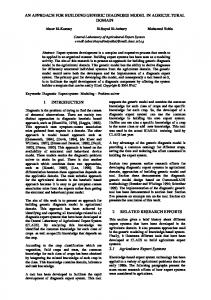
The input for the combination methods we have employed in this paper is the output of the single classifiers. For each class, the classifiers produce a soft value, i.e., a certain degree of support [13]. These outputs can be fuzzy, posterior probabilities, certainty, or possibility values [10]. Based on these soft outputs one can build a Decision Profile (DP). Formally, a DP for a given sample x can be defined as a L × C matrix, i.e., DP (x) = [D1 (x), D2 (x), ..., Dl (x), ..., DL (x)] in which Dl (x) = [dl,1 (x), dl,2 , ..., dl,c , ..., dl,C (x)]T , L is the number of classifiers, C is the number of classes, and dl,c (x) is the degree of support given by classifier Dl to class c [10, 13], as illustrates Fig. 1. After building support degrees for each input sample, a crisp value (the final label) can be assigned by using the maximum support value in the set, for instance.

Fig. 1: Decison Profile. Adapted and modified from [13].

According to Kuncheva [13], combiners are methods that use all predictions produced by two or more classifiers to build an accurate final decision. They can

be divided into “nontrainable” and “trainable” combiners. The “nontrainable” combiners have no need of training any parameter. They perform some basic operation (for instance: average, maximum, minimum and product) in the DP to produce new support values and, hence, a final decision. The purpose of the “trainable” combiners is to give more discriminant power to classifiers that have greater accuracy [13] when classifiers have different outputs. Weighted Average, Weighted Majority Vote (WMV), and other weighted approaches are based on this idea. In the following, we briefly describe the two linearly weighted combiners used in our proposed selection method, which, in turn, is described further. In this work, in particular, we use weighted linear combiners, from our previous works [19, 21]. Let us first define a Weighted Linear Combination (WLC). PL Given a sample x, let µc (x) = l=1 wl × dl,c (x) be the support for the class c, wl be the weight of the l-th classifier and dl,c (x) be the support of l-th classifier for the class c. The task of finding the best weights can be seen as an Integer Linear Programming (ILP) optimization problem, generated the WLC-ILP approach [21]. This problem requires the minimization (or maximization) of a linear form subject to linear inequality constraints. New supports for each class are built using the WLC and the weights found by running the simplex method. Then, a label is assigned, for a given sample x, as the index of the maximum support µc (x). The IBM CPLEX solver [12], a state-of-art ILP solver, is used as optimization routine. In [19], predictions of classifiers are also combined using a weighted linear combination of the DP, as stated above. However, the weights are found using a global search performed by a GA named WLC-GA. The fitness function was built based on the accuracy produced using the WLC in the dataset. A bit string representation encode the weights in individual chromosomes. Each weight can be a non-negative integer value between 0 and 127, which means that there are 7 bits in chromosome for each weight. 2.2

Search Methods

Many works have investigated methods for selecting subsets of classifiers rather than combining all classifiers [7, 8, 19, 22]. This selection aims at improving the performance of the combination, since it focuses on finding the subset of the most relevant classifiers. From a set of classifiers Cl, we apply search algorithms to select the subset of the best performing classifiers S, where |S| ≤ |Cl|. We can notice two important aspects: the search algorithm and the search criterion. Evolutionary Algorithms, such as Genetic Algorithms, attempt to find an optimal or near optimal global solution. More specifically Multi-Objective Genetic Algorithms seem to be a better option to the classifier selection problem due to the possibility of dealing with a population of solutions. Another important aspect is the choice of the most appropriate search criterion. Although there is no consensus, the role played by diversity is emphasized

in the literature. However, diversity and accuracy does not exhibit a strong relationship [4] and the estimated accuracy can not be replaced by diversity [9]. Our approach exploits a Multi-Objective Genetic Algorithm for searching. The search criteria used are the accuracy and the number of classifiers. We intend to reduce the number of classifiers, but also increase the accuracy. The final accuracy of the combination is the one obtained by either the WLC-ILP or WLC-GA combiners using the selected subsets of classifiers.

3

Multi-Objective Optimization Approach

In this section, we present the multi-objective remote sensed hyperspectral image classifier combiner (MORSHICC) based on genetic algorithm. We evolve a population of classifier combiners aiming at accuracy maximization and minimization of the number of classifiers. The latter objective searches for faster and less expensive combiners to efficiently classify large datasets. Each individual is a combiner which, in turn, is represented by a set of classifiers and its weights computed by a method, e.g., WLC-ILP or WLC-GA. The set of classifiers for combination contains twelve classification approaches as shown in Tables 1 and 2. We use a binary chromosome representation, in which each position (gene) on chromosome represents the presence (or absence) of a classifier. The population successively evolves through the generations following a tournament which randomly selects two individuals and then applies crossover and mutation rules. The binary selection is run six times such that twelve (M ) child individuals are generated. We use the one-point crossover, e.g., a point along the chromosome is randomly selected, then the pieces to the left of that point are exchanged between the chromosomes, producing a pair of offspring chromosomes as crossover operator, and bit inversion as mutation operator. We start with a randomly chosen initial population of size M , e.g., the number of classifier combiners used, in which the number of classification approaches in each individual also randomly varies. For each individual of the initial population, a combiner (WLC-ILP or WLC-GA) is run, and based on the classifier combiner generated, the pair (classification accuracy, number of classifiers) is computed. Note that either the WLC-ILP or WLC-GA is adopted during the optimization process. The evolution step is defined in terms of two objectives: maximizing the classification accuracy and minimizing the number of classifiers. This step relies on the concept of dominance: a point is said to be dominated if it is worse than another point in at least one objective, while not being better than that point in any other objective. The Pareto-set is the set that contains no dominated solution, thus it consists of points that are not simultaneously worse than any other point in both objectives. More specifically, a generation of the MORSHICC genetic algorithm works as presented in Algorithm 1. Note that the initial population (generation zero) is first evaluated (i.e., combiners’ computation). Then, it is submitted to the Generation step. At the beginning of each generation, we create more M child

Algorithm 1 Generation step of our MORSHICC 1: 2: 3: 4: 5: 6: 7: 8: 9: 10: 11: 12: 13:

input: current: set of M evaluated individuals child ← bin. select. on current and mutation & crossover for each ind ∈ child do {evaluating every child} (acc., #class.) ←WLC-ILP (or WLC-GA) of ind current ← current ∪ child {|current| = 2 × M } next ← ∅ repeat {Pareto-set evaluation procedure} best ← non-dominance set from current next ← next ∪ best current ← current − best until |next| ≤ M remove extra individuals output: next: set of M evolved and evaluated individuals

individuals using binary selection and crossover/mutation operators (lines 2). The child individuals are evaluated (lines 3-4) and joined to the parent individuals updating the so called current generation set to 2M individuals (line 5). The next generation set (output) is composed of individuals that survive to the recursive Pareto-set evaluation procedure (lines 6-11). The Pareto-set of the current generation set (line 8) is inserted into the next generation set (line 9), which is initially empty (line 6). The current Pareto-set (best) is removed from the current generation set (line 10). The process of computing a new Pareto-set of the remaining individuals is repeated (lines 8-10) until the next generation set contains M individuals. If eventually the last Pareto-set collects individuals that extrapolates the M size limit of the generation set, among the last inserted individuals, the ones with highest accuracy standard deviation3 are removed, so that the output set reach exactly M individuals (lines 12-13). The evolution (generation) process is repeated until a predetermined maximum number of generations is reached. This procedure is similar to the “NonDominated Sorting” selection operator, which is employed in the NSGA-II [6]. It is noticeable that the final subset of classifier combiners is reprocessed such that only non-dominated solutions remain.

4

Experimental Results and Discussion

The classification approaches selected for combination should constitute a diverse set and provide additional information. For such aim we used data representations such as: Pixelwise [15]; Extend Morphological Profile (EMP) [1]; and Feature Extraction by Genetic Algorithms (FEGA) [20]. For classification, we used well-known learning algorithms such as Support Vector Machines (SVM) [15], with Radial Basis Function (RBF) and Linear kernels, Multilayer Perceptron Neural Network (MLP) [1], and k-Nearest Neighbor (KNN) [5]. The full set of 3

Each combiner is evaluated using several training/testing sets

Table 1: IP dataset: classification approaches. Identifier 1 2

Classification Approaches EM P

Train Accuracy (%) 10% 15%

RBF -SV M 88.77-(±0.39) 90.88-(±0.29)

P ixelW ise RBF -SV M 80.38-(±0.44) 83.51-(±0.29)

3

F EGA

4

EM P

5 6

RBF -SV M 76.27-(±0.50) 78.99-(±0.34) M LP

81.60-(±0.76) 82.62-(±0.67)

P ixelW ise

M LP

73.04-(±0.75) 76.83-(±0.48)

F EGA

M LP

72.26-(±0.80) 75.14-(±0.64)

7

EM P

kN N

83.94-(±0.34) 86.62-(±0.38)

8

P ixelW ise

kN N

67.28-(±0.44) 69.40-(±0.33)

9

F EGA

kN N

61.76-(±0.62) 63.66-(±0.38)

10

EM P

linSV M

79.10-(±0.55) 80.14-(±0.43)

11

P ixelW ise

linSV M

77.17-(±0.50) 80.55-(±0.39)

12

F EGA

linSV M

72.96-(±0.59) 75.67-(±0.49)

classifiers used for combination contains twelve classification approaches (Tables 1 and 2). Experiments were carried out in two training set scenarios, i.e., with 10% and 15% of samples using the well-know Indian Pines (IP) and Pavia University (PU) datasets. In both scenarios, the testing set were adjusted to 85% of unseen samples for a fair comparison of the obtained effectiveness. During the MORSHICC evolution, each individual (classifier combiner) was run 30 times using 30 different training and testing sets randomly created. Mean and variances of these experiments were used to compute the confidence intervals of each combiner using a 0.05 confidence level. For each run of each evaluated combiner, it is important to note that 50% of the training data is used for initially train the classifiers and the remaining 50% used for weights estimation in order to avoid biased and specialized weights, and in a second training phase the classifiers are retrained with the entire training set. Note that these all subsets (training+testing) were initially created and then used in all experiments such that a fair comparison can be performed. MORSHICC approach setup: We set the generation number to 10 with a population of 12 individuals. We evaluated only 120 individuals during the evolution process due to the high computation cost of our approach, which took almost one week for both datasets using a personal computer with Intel(R) Core(TM) i5-2450M processor and 4 GB of main memory with Ubuntu 12.04 Operating System. We used 12 bits to represent the presence/absence of each classification approach in combination, and the probabilities of crossover and mutation to 80% and 0.9%, respectively.

Table 2: PU dataset: classification approaches. Identifier 1 2

Classification Approaches EM P

Train Accuracy (%) 10% 15%

RBF -SV M 97.20-(±0.11) 97.56-(±0.08)

P ixelW ise RBF -SV M 93.17-(±0.13) 93.50-(±0.10)

3

F EGA

4

EM P

5 6

RBF -SV M 90.87-(±0.22) 91.39-(±0.11) M LP

94.42-(±0.50) 94.48-(±0.74)

P ixelW ise

M LP

92.43-(±0.20) 92.91-(±0.14)

F EGA

M LP

89.70-(±0.27) 90.04-(±0.19)

7

EM P

kN N

95.56-(±0.12) 96.23-(±0.08)

8

P ixelW ise

kN N

84.99-(±0.17) 85.82-(±0.13)

9

F EGA

kN N

88.31-(±0.18) 89.06-(±0.11)

10

EM P

linSV M

90.72-(±0.16) 91.31-(±0.13)

11

P ixelW ise

linSV M

90.96-(±0.18) 91.10-(±0.13)

12

F EGA

linSV M

87.52-(±0.22) 87.61-(±0.13)

Table 3: Results for IP dataset using 10% training set. training set 10%

Classifiers’ ID

Number of Accuracy Confidence Classifiers (%) Interval

WLC-ILP

1-2-3-4-5-6-7-8-9-10-11-12

12

89.57

0.80

WLC-GA

1-2-3-4-5-6-7-8-9-10-11-12

12

89.72

0.52

MORSHICC in WLC-ILP

1-2-4-5-7-11-12

7

90.15

0.46

MORSHICC in WLC-GA

1-2-4-6-7-8-10-11

8

91.12

0.29

Best Individual Classifier

1

1

88.77

0.39

In the following, the analysis for claiming statistically significance takes into account the confidence intervals and mean accuracies reported in Tables 3, 4, 5, and 6. In these same tables, from the Pareto’s front combiners obtained for MORSHICC in WLC-ILP and WLC-GA, we choose to report the best mean accuracies obtained by the combiners which are the ones with the largest number of classifiers. For the IP dataset using 10% of training samples, in Table 3, it is shown that our approaches achieved significantly better results than the best individual clas-

Table 4: Results for IP dataset using 15% of training set. training set 15%

Classifiers’ ID

Number of Accuracy Confidence Classifiers (%) Interval

WLC-ILP

1-2-3-4-5-6-7-8-9-10-11-12

12

91.55

0.62

WLC-GA

1-2-3-4-5-6-7-8-9-10-11-12

12

91.63

0.54

MORSHICC in WLC-ILP

1-2-3-4-7-10-11

7

93.00

0.24

MORSHICC in WLC-GA

1-2-4-5-7-8-11

7

93.30

0.21

Best Individual Classifier

1

1

90.88

0.29

sifier. Also observe that the MORSHICC approach in the WLC-ILP produced statistically similar accuracy, and the MORSHICC approach in the WLC-GA produced statically better accuracy when compared with their respective combiner using all classification approaches. Anyway in both cases MORSHICC approach employed fewer classifier. For the IP dataset using 15% of training samples, our approaches have also achieved significantly better results than the best individual classifier accuracy as shown in Table 4. Moreover, in this scenario, the MORSHICC approaches produced significantly better accuracies with fewer classifiers when compared to both the WLC-ILP and WLC-GA combiners using all classifiers. Note that the classification accuracies obtained using 15% for training the classifiers are significantly higher than when using 10%. Figure 2 shows the graphs of the Pareto’s fronts produced by our MORSHICC approach training in 10% and 15% of training samples and tested in 85% of samples. It is important to claim that the individual approach 1 (EM P + RBF -SV M ), which has higher accuracy, is present in most combinations that generated the Pareto’s fronts. By observing and comparing the red points (combiners) of each graph of the Pareto’s front, it is possible to see that smaller combiners (few classifiers) can also produce higher accuracies with no statistically difference to the best combiners. This information is useful when faster combiners (with low computational cost) are required. For the PU dataset, using 10% and 15% of training samples, Tables 5 and 6, respectively, show that the MORSHICC approach in the WLC-GA combiner achieved significantly better results than the best individual classifier. However its result is not statistically better if compared with the one obtained by the WLC-GA approach using all combiners. Moreover, the MORSHICC in the WLCILP performed poorly than the best individual combiner and also with respect to the WLC-ILP approach using all combiners. Notice that the accuracy improvement obtained in this dataset is smaller if compared with the obtained results

100

98

98

96

96

94

94

Accuracy

Accuracy

100

92 90 88

92 90 88

86

86

84

84

82

82

80

0

1

2

3

4

5

6

7

8

9

10

11

80

12

0

1

2

3

Number of Classifiers

5

6

7

8

9

10

11

12

11

12

(b) WLC-ILP/Training Set: 15%.

100

100

98

98

96

96

94

94

Accuracy

Accuracy

(a) WLC-ILP/Training Set: 10%.

92 90 88

92 90 88

86

86

84

84

82 80

4

Number of Classifiers

82 0

1

2

3

4

5

6

7

8

9

10

Number of Classifiers

(c) WLC-GA/Training Set: 10%.

11

12

80

0

1

2

3

4

5

6

7

8

9

10

Number of Classifiers

(d) WLC-GA/Training Set: 15%.

Fig. 2: Pareto’s fronts for IP dataset. Blue bars stand for the confidence intervals.

for the IP dataset since here there is few room for improvement, i.e., the best individual classifier produces less than 3% of error. As a possible consequence of this fact, observe that the best results obtained for 15% (the MORSHICC in the WLC-GA) is not significantly better than the one obtained for 10% (the MORSHICC in the WLC-GA), even it is slightly higher. Figure 3 shows the graphs of the Pareto’s front produced by our approach for the PU dataset using 10% and 15% of training samples. We can observe the same conclusions we had in Figure 2 (IP dataset), however here with higher accuracies. In general (both datasets), the MORSHICC approaches in the WLC-GA combiner produces higher accuracies than the ones MORSHICC approaches in the WLC-ILP method, although they are not necessarily better in terms of statistical significance. This negative result of the WLC-IP method can be justified by the numerical instability faced by it for solving the optimization problem. Nonetheless the WLC-ILP method is in average 20 times faster than the WLCGA combiner for estimating the final weights as shown in [21].

Table 5: Results for PU dataset using 10% of training set. Approaches

Classifiers’ ID

Number Accuracy Confidence Classifiers (%) Interval

WLC-ILP

1-2-3-4-5-6-7-8-9-10-11-12

12

97.73

0.18

WLC-GA

1-2-3-4-5-6-7-8-9-10-11-12

12

97.55

0.62

MORSHICC in WLC-ILP

1-4-7-9-11

5

97.11

0.30

MORSHICC in WLC-GA

1-2-5-7-10-11-12

7

98.00

0.09

Best Individual Classifier

1

1

97.20

0.11

Table 6: Results for PU dataset using 15% of training set.

5

training set 15%

Classifiers’ ID

Number Accuracy Confidence Classifiers (%) Interval

WLC-ILP

1-2-3-4-5-6-7-8-9-10-11-12

12

98.12

0.24

WLC-GA

1-2-3-4-5-6-7-8-9-10-11-12

12

97.87

0.11

MORSHICC in WLC-ILP

1-2-3-4-5-7-11

7

97.28

0.40

MORSHICC in WLC-GA

1-2-3-5-7-11

6

98.44

0.79

Best Individual Classifier

1

1

97.56

0.08

Conclusions

In this paper, we have presented a multi-objective remote sensed hyperspectral image classifier combiner (MORSHICC) approach based on genetic algorithm to determine the Pareto’s front. Our aim is to use the Pareto’s front to determine the set of best combiners. We have modeled the problem according to two objectives: maximization of accuracy and minimization of the number of classifiers used in the combiner. Experimental analysis shows that MORSHICC not only produces an ensemble with a very small set of classifiers but also improves the final accuracy results. Furthermore, the obtained ensembles may achieve more accurate thematic maps for real and large datasets in a short time. Future work includes the application of the proposed techniques in real world problems, such as automatic agricultural crop recognition.

100

98

98

96

96

94

94

Accuracy

Accuracy

100

92 90 88

92 90 88

86

86

84

84

82

82

80

0

1

2

3

4

5

6

7

8

9

10

11

80

12

0

1

2

3

Number of Classifiers

5

6

7

8

9

10

11

12

11

12

(b) WLC-ILP/Training Set: 15%.

100

100

98

98

96

96

94

94

Accuracy

Accuracy

(a) WLC-ILP/Training Set: 10%.

92 90 88

92 90 88

86

86

84

84

82 80

4

Number of Classifiers

82 0

1

2

3

4

5

6

7

8

9

10

Number of Classifiers

(c) WLC-GA/Training Set: 10%.

11

12

80

0

1

2

3

4

5

6

7

8

9

10

Number of Classifiers

(d) WLC-GA/Training Set: 15%.

Fig. 3: Pareto’s fronts for PU dataset. Blue bars stand for the confidence intervals.

Acknowledgements The authors thank UFOP and funding Brazilian agencies CNPq, Fapemig and CAPES.

References 1. Benediktsson, J., Palmason, J., Sveinsson, J.: Classification of hyperspectral data from urban areas based on extrended morphological profiles. IEEE Trans. on Geoscience and Remote Sensing (TGARS) 43(3), 480–491 (2005) 2. Benediktsson, J.A., Chanussot, J., Fauvel, M.: Multiple classifier systems in remote sensing: From basics to recent developments. In: International Workshop on Multiple Classif. Syst. pp. 501–512 (2007) 3. Benediktsson, J.A., Chanussot, J., Moon, W.M.: Very high-resolution remote sensing: Challenges and opportunities [point of view]. Proceedings of the IEEE 100(6), 1907–1910 (2012) 4. Brown, G., Kuncheva, L.I.: GOOD and BAD diversity in majority vote ensembles. In: International Workshop on Multiple Classif. Syst. vol. LNCS 5997, pp. 124–133 (2010)

5. Cover, T., Hart, P.: Nearest neighbor pattern classification. IEEE Trans. on Information Theory 13(1), 21 –27 (january 1967) 6. Deb, K.: Multi-objective optimisation using evolutionary algorithms: An introduction. In: Multi-objective Evolutionary Optimisation for Product Design and Manufacturing, pp. 3–34. Wiley (2011) 7. Dos Santos, J.A., Faria, F.A., da S Torres, R., Rocha, A., Gosselin, P.H., PhilippFoliguet, S., Falcao, A.: Descriptor correlation analysis for remote sensing image multi-scale classification. In: Pattern Recognition (ICPR), 2012 21st International Conference on. pp. 3078–3081 (2012) 8. Faria, F.A., dos Santos, J.A., Rocha, A., da S. Torres, R.: A framework for selection and fusion of pattern classifiers in multimedia recognition. Pattern Recognition Letters 39, 52–64 (2014) 9. Gabrys, B., Ruta, D.: Genetic algorithms in classifier fusion. Applied soft computing 6(4), 337–347 (2006) 10. Ghosh, A., Shankar, B., Bruzzone, L., Meher, S.: Neuro-fuzzy-combiner: an effective multiple classifier system. Int. J. of Knowledge Engineering and Soft Data Paradigms 2(2), 107–129 (2010) 11. Hadjitodorov, S.T., Kuncheva, L.I., Todorova, L.P.: Moderate diversity for better cluster ensembles. Information Fusion 7(3), 264–275 (2006) 12. ILOG S.A.: CPLEX 12.5 User’s Manual (2012) 13. Kuncheva, L.: Combining Pattern Classifiers: Methods and Algorithms. 2004. Wiley-Interscience (2004) 14. Licciardi, G., Marpu, P., Chanussot, J., Benediktsson, J.: Linear versus nonlinear PCA for the classification of hyperspectral data based on the extended morphological profiles. IEEE Geoscience and Remote Sensing Letters (GRSL) 9(3), 447–451 (2012) 15. Melgani, F., Bruzzone, L.: Classification of hyperspectral remote sensing images with support vector machines. IEEE Trans. on Geoscience and Remote Sensing (TGARS) 42(8), 1778–1790 (2004) 16. Plaza, A., et al.: Recent advances in techniques for hyperspectral image processing. Remote Sensing Environment 113(1), 110–122 (2009) 17. Polikar, R.: Ensemble based systems in decision making. IEEE Circuits and Systems Magazine 6(3), 21–45 (2006) 18. Prasad, S., Bruce, L.M., Chanussot, J.: Optical Remote Sensing: Advances in Signal Processing and Exploitation Techniques, vol. 3. Springer (2011) 19. Santos, A.B., de A. Ara´ ujo, A., Menotti, D.: Combining multiple classification methods for hyperspectral data interpretation. IEEE Journal of Selected Topics in Applied Earth Observations and Remote Sensing 6(3), 1450–1459 (2013) 20. Santos, A.B., de S. Celes, C.S.F., de A.Arajo, A., Menotti, D.: Feature selection for classification of remote sensed hyperspectral images: A filter approach using genetic algorithm and cluster validity. In: The 2012 International Conference on Image Processing, Computer Vision, and Pattern Recognition (IPCV). vol. 2, pp. 675–681 (2012) 21. Tinˆ oco, S., Santos, A., Santos, H., dos Santos, J.A., Menotti, D.: Ensemble of classifiers for remote sensed hyperspectral land cover analysis: An approach based on linear programming and weighted linear combination. In: IEEE Int. Geoscience and Remote Sensing Symposium (IGARSS). pp. 4082–4085 (2013) 22. Zhang, L., Zhang, L., Tao, D., Huang, X.: On combining multiple features for hyperspectral remote sensing image classification. IEEE Trans. on Geoscience and Remote Sensing (TGARS) 50(3), 879–893 (2012)