Int. J. Advanced Operations Management, Vol. X, No. Y, xxxx
A multi objective solid transportation problem in fuzzy, bi-fuzzy environment via genetic algorithm Sutapa Pramanik Deulia Balika Bidyamandir, Deulia, Purba Midna Pur-721154, West Bengal, India E-mail:
[email protected]
D.K. Jana* Department of Applied Sciences, Haldia Institute of Technology, Haldia, Purba Midna Pur-721657, West Bengal, India Fax: 03224-252800 E-mail:
[email protected] *Corresponding author
K. Maity Department of Mathematics, Mugberia Gangadhar Mahavidyalaya, Mugberia, Purba Medinipur-721425, West Bengal, India Fax: 03224-252800 E-mail:
[email protected] Abstract: In this paper, we concentrate on developing a bi-fuzzy multi objective transportation problem (MOSTP) according to bi-fuzzy expected value method (EVM). In a transportation model, the available discount is normally offered on items/criteria, etc., in the form all unit discount (AUD) or incremental quantity discount (IQD) or combination of these two. Here transportation model is considered with fixed charges and vehicle costs where AUD, IQD or combination of AUD and IQD on the price depending upon the amount is offered and varies on the choice of origin, destination and conveyance. To solve the problem, multi objective genetic algorithm (MOGA) based on Roulette wheel selection, arithmetic crossover and uniform mutation has been suitably developed and applied. To illustrate the models, numerical examples have been presented. Here, two types of problems are introduced and the corresponding results are obtained. To provide better customer service, the entropy function is considered. Keywords: bi-fuzzy; genetic algorithm; solid transportation problem; STP; entropy.
Copyright © 200x Inderscience Enterprises Ltd.
1
2
S. Pramanik et al. Reference to this paper should be made as follows: Pramanik, S., Jana, D.K. and Maity, K. (xxxx) ‘A multi objective solid transportation problem in fuzzy, bi-fuzzy environment via genetic algorithm’, Int. J. Advanced Operations Management, Vol. X, No. Y, pp.000–000. Biographical notes: Sutapa Pramanik is an Assistant Teacher in Deulia Balika Bidyamandir, Deulia, Purba Medinipur, India. She received her MSc in Applied Mathematics from Vidyasager University. She also qualified NET, GATE, SET examinations. Her research interests are transportation problem in fuzzy, fuzzy rough and uncertain environments. She has published many research papers in reputed international journals. D.K. Jana is an Assistant Professor in Haldia Institute of Technology, Haldia, Purba Medinipur, and West Bengal India. He received his MSc in Applied Mathematics from Vidyasager University. His research interests are in inventory and optimal control of production systems in fuzzy, fuzzy rough and uncertain environments. He published many research papers in reputed international journals such as JOS, IJOR, OPSEARCH, etc. K. Maity received his PhD in Applied Mathematics from Vidyasagar University in 2006. He is a Lecturer in the Department of Mathematics, Mugberia Gangadhar Mahavidyalaya, Purba Medinipur. His research and development efforts focus on operational research, optimal control theory, fuzzy mathematics and fuzzy logic. He published many research papers in reputed international journals such as EJOR, MCM, FODM, AJMMS, Information Sciences, etc.
1
Introduction
Generally speaking, uncertainty is common to all real-life problems for example randomness, fuzziness and roughness. Since Zadeh (1965) introduced the fuzzy set in 1965, fuzzy set theory has been well developed and applied to a wide variety of real problems. After that, Liu and Liu (2003) have developed a class of fuzzy random optimisation: expected value models. Maity et al. (2008) have developed a production recycling model with imprecise holding cost. Production of defective units is a natural phenomenon in a production process. Bi-fuzzy sets were originally presented by Zadeh (1971) and were further elaborately by Gottwald (1979), Mendel and John (2002), Pandian and Anuradha (2010), others. But, till now, none has considered MOSTP problem with fuzzy fixed charge, vehicle cost and price discounted varying charge and bi-fuzzy total sources, destinations and conveyances. The solid transportation problem (STP) was first introduced by Haley (1962) in 1962, in which three kinds of constraints are taken into consideration, that is, source constraint, destination constraint and conveyance capacity constraint. The STP degenerates into the classical transportation problem as the number of conveyance is only one. In recent years, there have been numerous papers in this area. Some papers only minimises the total transportation cost. For example, Ojha et al. (2010) and Tao and Xu (2012) considered a STP for an item with fixed charge, vehicle cost and price discounted varying charge. To solve the problem, the genetic algorithm (GA), which is based on Roulette wheel selection, arithmetic crossover and uniform mutation, was suitably developed and
Comment [t1]: Author: Please rewrite the sentence to make the intended meaning clear to readers.
A multi objective solid transportation problem
3
applied. However, in practical programming problems, the decision maker (DM) usually needs to optimise several objectives. Unfortunately, the objectives are often conflicting and incommensurable. Thus, the DM cannot obtain the optimal values of all the objectives simultaneously. The growing literature of STP focuses on multiple objective problems, that is, multiple objective solid transportation problems (MOSTPs). For example: Bit et al. (1993) used a fuzzy programming approach to solve a MOSTP; Ida et al. (1996) presented a neural network method to solve a MOSTP. Tao and Xu (2012) have developed a class of rough multiple objective programming and its application to STP. In today’s highly competitive market the pressure on organisations to find the better ways to create and deliver values to customers is increasing more and more. How and when to send the products to the customers in the quantities they want in a cost-effective manner has become more challenging in terms of price discount [all unit discount (AUD) and/or incremental quantity discount (IQD)] on the unit transportation cost. There is a similarity to economic ordered quantity model for such a discount (cf. Maiti and Maiti, 2008). To solve the STP, the GA, which is based on Roulette wheel selection, arithmetic crossover and uniform mutation, was suitably developed and applied. However, in practical programming problems, the DM usually needs to optimise several objectives. Unfortunately, the objectives are often conflicting and incommensurable. Thus, the DM cannot obtain the optimal values of all the objectives simultaneously. A growing body of literature of STP focuses on multiple objective problems, that is, MOSTPs. For the solution of decision-making problems, there are some inherent difficulties in the traditional direct and gradient-based optimisation techniques used for this purpose. Normally, these methods 1
are initial solution dependent
2
get stuck to a sub-optimal solution
3
are not efficient in handing problems having discrete variables
4
cannot be efficiently used on parallel machines
5
are not universal, rather problem dependent.
To overcome these difficulties, recently GAs are used for optimisation of decision making problems. GAs (Goldberg, 1989; Vignaux and Michalewicz, 1991) are adaptive computational procedures modelled on the mechanics of natural genetic systems. They exploit the historical information to speculate on new offspring with expected improved performance. These are executed iteratively on a set of coded solutions (called population) with three operators – selection/reproduction, crossover and mutation. One set of these three operators is known as a generation in the parlance of GA Since a GA works simultaneously on a set of solutions, it has very little chance to get suck at local optimum. Here, the resolution of the possible search space is increased by operating on potential solutions and not on the solutions themselves. Further, this search space need not be continuous. Recently, GAs have been applied in different areas like neural network, travelling salesman, scheduling, numerical optimisation (Vignaux and Michalewicz, 1991), inventory (Mandal and Maiti, 2000; Maiti and Maiti, 2008; Pramanik and Roy, 2008), etc. Recently, Ojha et al. (2010) have developed a STP for an
4
S. Pramanik et al.
item with fixed charge, vehicle cost and price discounted varying charge using GA. But none can consider MOSTP in imprecise environment. In this paper, a multi objective STP with discounted costs, fixed charges and vehicle costs are formulated as a liner programming problem. The discounted costs are in the form of AUD, IQD and combination of AUD and IQD. Here AUD, IQD or combination of these two discounts on purchasing price with two price breaks are considered. Here, the transportation costs, resources, demands at various centres and conveyance capacities, times for different modes of transport between origins and destinations are bi-fuzzy. The STP has been formulated in two different ways with and without entropy function following Shannon’s measure of entropy. Then the multi objective STPs are solved using MOGA and the results of these two types of problems are tabulated.
2
Necessary knowledge about fuzzy, bi-fuzzy sets and bi-fuzzy EVM
In this section, we recall some basic knowledge of fuzzy set theory, bi-fuzzy and bi-fuzzy EVM.
2.1 Fuzzy set A fuzzy set is a class of objects in which there is no sharp boundary between those objects that belong to the class and those that do not. Let X be a collection of objects and x be an element of X, then a fuzzy set A in X is a set of ordered pairs A = {( x, μ A ( x)) / x ∈ X } where μ A ( x) is called the membership function or grade of
membership of x in A which maps X to the membership space M which is considered as the closed interval [0, 1]. Fuzzy number: A fuzzy number A is a convex normalised fuzzy set on real line ℜ such that 1
it exists exactly one x0 ∈ ℜ with μ A ( x0 ) = 1 (x0 is called the mean value of M )
2
μ A ( x) is piecewise continuous.
Example: In particular if A = (a1 , a2 , a3 ) be a triangular fuzzy number (TFN) (cf. Figure 1) then μ A ( x) is defined as follows ⎧ x – a1 ⎪a – a ⎪⎪ 2 1 a −x μ A ( x) = ⎨⎪ 3 a −a ⎪ 3 2 ⎪⎩0
for a1 ≤ x < a2 for a2 < x ≤ a3 otherwise
where a1, a2 and a3 are real numbers.
A multi objective solid transportation problem Figure 1
5 Comment [t2]: Author: Please confirm if you are satisfied with the resolution of this amended Figure 1 (in EPS file). If not, kindly then please provide us with another clear and readable version of this figure in any format you could provide us.
Triangular fuzzy number
Please also note that the other version of Figure 1 (in PNG file) that you provided us is more unreadable/vague than the EPS file format.
Lemma 1: Let a = (a1 , a2 , a3 ) be a triangular fuzzy number and ρ is a crisp number. The expected value of a is 1 [(1 – ρ)a1 + a2 + ρa3 ] , 0 < ρ < 1. 2 a + 2a2 + a3 , ρ = 0.5. = 1 4
E[a ] =
(1)
Proof: The proof of the Lemma 1 is in Liu and Liu (2003).
2.2 Bi-fuzzy set Generally speaking, a level 2 fuzzy set is a fuzzy set in which the elements are also fuzzy sets, and the bi-fuzzy variable is a fuzzy variable with fuzzy parameters. Level 2 fuzzy sets were originally presented by Zadeh (1971). Such sets are fuzzy sets whose elements themselves are ordinary fuzzy sets. They are very useful in circumstances where it is difficult to determine some elements for a fuzzy set.
Definition 1: In Mendel and John (2002), a type 2 fuzzy set, denoted A, is characterised by a type 2 membership function μ A ( x, u ), where x ∈ X and u ∈ Jx) ⊆ [0, 1], i.e.,
{
}
V = (V , μV (V ) ) | ∀x ∈ Γ(U ) : μV > 0
(2)
where each ordinary fuzzy set V is defined by
V = {( x, μV ( x) ) | ∀x ∈ U : μV > 0}
(3)
For convenience, the membership grades μV (V ) of the fuzzy sets .V ∈ Γ(U ) are called ‘outer-layer’ membership grades, whereas the membership grades μV ( x) of the elements x ∈ U are called inner-layer membership grades. Since level 2 fuzzy sets are still fuzzy sets, their mathematical behaviour is defined by the fuzzy set operators. Type 2 fuzzy sets were introduced by Zadeh (1975) as another extension of the concept of an ordinary fuzzy set, and it was elaborated by Mendel and John (2002). Such
6
S. Pramanik et al.
sets are fuzzy sets whose membership grades them as ordinary fuzzy sets. They are very useful in circumstances where it is difficult to determine an exact membership function for a fuzzy set. Normally speaking, a Fu-Fu variable (bi-fuzzy) is a fuzzy variable under fuzzy environment. Example: ξ = ( sL , ξ , sR ) with ρ = (ρL, ρM, ρR) is called Fu-Fu variable (cf. Figure 2), if the outer-layer and inner-layer membership functions are as follows ⎧⎛ x – sL ⎞ ⎪⎜ ⎟ if sL ≤ x ≤ ρ ⎪⎝ ρ – sL ⎠ ⎪ μξ ( x) = ⎨0 otherwise ⎪ s –x ⎞ ⎪⎜⎛ R if ρ ≤ x ≤ sR ⎪⎩⎝ sR – ρ ⎟⎠ and ⎧⎛ x′ – ρL ⎪⎜ ⎪⎝ ρM – ρL ⎪ μ ρ ( x ) = ⎨0 ⎪ ρ – x′ ⎪⎛ R ⎪⎩⎜⎝ ρR – ρM
⎞ ⎟ if ρL ≤ x′ ≤ ρM ⎠ otherwise ⎞ ⎟ if ρM ≤ x′ ≤ ρR ⎠
where ρ is the centre of ξ , which is a triangular fuzzy variable, sL ∈ R and sR ∈ R are the smallest possible value and the largest possible value of ξ , ρL ∈ R, ρM ∈ R and ρR ∈ R are the smallest possible value, the most promising value and the largest possible value of ρ respectively. Figure 2
Triangular bi-fuzzy variable (see online version for colours)
Comment [t3]: Author: Please confirm if you are satisfied with the resolution of this amended Figure 2 (in EPS file). If not, kindly then please provide us with another clear and readable version of this figure in any format you could provide us. Please also note that the other version of Figure 2 (in PNG file) that you provided us is more unreadable/vague than the EPS file format.
Lemma 2: The expected value for the bi-fuzzy variable c = (l1 , c , r1 ) with c = (l2 , c, r2 ) we obtain that
A multi objective solid transportation problem E [c ] = c +
( r1 + r2 ) – ( l1 + l2 )
7 (4)
4
Proof: The proof of the Lemma 2 is in Xu and Zhou (2009) in Section 4, p.276. Lemma 3: Assume that ξ and η are fuzzy/bi-fuzzy variables with finite expected values. Then for any real numbers a and b, we have E[aξ + bη] = aE[ξ ] + bE[η]
(5)
Proof: The proof of the Lemma 3 is in Xu and Zhou (2009).
2.3 General model for bi-fuzzy EVM First we give the general model of Fu-Fu multi-objective decision making model as follows, ⎧ ⎪ Min ⎪ ⎨ ⎪ s.t ⎪⎩
( ) ( ) , f ( x, ξ ) ⎧⎪ ( g x, ξ ) ≤ 0, r = 1, 2,… , p ⎨ f1 x, ξ , f 2 x, ξ ,
m
(6)
r
⎪⎩ x ∈ X
If ξ is a Fu-Fu vector, x = (x1, x2,···,xn) is decision vector, then the objective function fi ( x, ξ ) and constraint functions g r ( x, ξ ) are also Fu-Fu variables, i = 1, 2,···,m,
r = 1, 2,···,p. In order to rank Fu-Fu objective fi ( x, ξ ), we may employ the expected value operator to deal with the objective functions and constraints, and we can get the following model (6). For the expected value of the objective E[ fi ( x, ξ )], i = 1, 2,···,m, it means that the larger the expected returns E[ fi ( x, ξ )], the better the decision x. The first type of Fu-Fu decision-making model is expected value multi-objective decision-making model in which the underlying philosophy is based on selecting the decision with maximum expected objective values. ⎧ ⎪ Min ⎪ ⎨ ⎪ s.t ⎪ ⎩
( ) ( )
( )
( )
⎡ ⎤ ⎡ ⎤ ⎡ ⎤ E ⎣ f1 x, ξ ⎦ , E ⎣ f 2 x, ξ ⎦ , , E ⎣ f m x, ξ ⎦ ⎧ ⎡ ⎪ E g r x, ξ ⎤⎦ ≤ 0, r = 1, 2,… , p ⎨ ⎣ ⎪⎩ x ∈ X
(7)
Theorem 1: If α rje 1 , α rje 2 , β rje 1 , β rje 2 are left and right spreads of erj (θ ) and erj (θ ), α rb1 ,
α rb2 , β rb1 , β rb2 are left and right spreads of br (θ ) and br (θ ), r = 1, 2,···,p, j = 1, 2,···,n, the basis function L, R: [0, 1] → [0, 1] are monotone decreasing continuous function, and it satisfies L(1) = R(1) = 0, L(0) = R(0) = 1 and the LR fuzzy variable is specified as the triangular fuzzy variable and R–1(θi) = 1 – θi, R–1(ηi) = 1 – ηi. For any j = 1, 2,···,n, and if erj (θ ) and br (θ ) are independent fuzzy variables. Then
8
S. Pramanik et al.
{
{
} }
Pos θ | Pos erjT (θ ) x ≤ br (θ ) ≥ θr ≥ ηr
is equivalent to R –1 ( θr ) β rb1 + L–1 ( θr ) α reT1 x – erT x + br + L–1 ( ηr ) (α reT1 x + β rb2 )
Proof: The proof of the Theorem 1 is in Xu and Zhou (2009) in p.254. Theorem 2: Assume that the Fu-Fu variable eij and br is as same as the assumption in Theorem 1, i = 1, 2,···,m, j = 1, 2,···,n. For confidence level δi, γi ∈ [0, 1], i = 1, 2,···,m. Then
{
{
} }
Nec δ | Nec erj (δ )T x ≤ br (δ ) ≥ δr ≥ γr
is equivalent to br – erT x – L–1 (1 – γr ) (α rb2 + β reT2 x ) – L–1 (1 – δr ) δrb1 – R –1 ( δr ) β reT1 x ≥ 0
Proof: The proof of the Theorem 1 is in Xu and Zhou (2009) in p.257.
3
Assumptions and notation
3.1 Notation In this STP, the following notation 1
m = number of sources of the transportation problem
2
n = number of demands of the transportation problem
3
K = number of conveyances, i.e., different modes of the transportation problem
4
Oi = origins of the transportation problem
5
Dj = destination of the transportation problem
6
Ek = conveyances of the transportation problem
7
ai = bi-fuzzy amount of a homogeneous product available at ith origin
8
b j = bi-fuzzy demand at jth destination
9
ek = bi-fuzzy amount of product which can be carried by kth conveyance
10 fijk = the fixed charge of the transportation problem 1 = fuzzy unit transportation cost from ith origin to jth destination by kth 11 Cijk
conveyance 2 12 Cijk = fuzzy transportation time which amount transported from ith origin to jth
destination by kth conveyance
A multi objective solid transportation problem
9
13 h(x) = the probability that X is in the state x.
3.2 Assumptions In this STP, the following assumptions are made. 1
The total vehicle cost
⎧ s.V G ( xijk ) = ⎨ ⎩( s + 1).V
if s.Vc = xijk
2
s = [xijk / Vc], Vc = vehicle capacity and V = vehicle cost.
3
The unit transformation cost under AUD scheme:
1 Cijk
⎧ p1ijk ⎪p ⎪ 2ijk ⎪⎪ =⎨ ⎪ ⎪ ptijk ⎪ ⎪⎩ p(t +1)ijk
if 0 < xijk < R1 if R1 ≤ xijk < R2
(9) if R(t –1) ≤ xijk < Rt if Rt ≤ xijk
where p1ijk , p2ijk , p3ijk , 4
, ptijk , p(t +1)ijk are all fuzzy unit cost.
IQD: The unit-transportation cost under IQD system is p1ijk for 0 < xijk < R1, p2ijk for an additional quantity over R1 but less then R2 and so on, lastly p(t +1)ijk for any additional quantity over Rt. Thus, unit transportation cost becomes
C1ijk
4
(8)
Otherwise
⎧ p1ijk ⎪ ⎪⎡⎣ p1ijk R1 + p2ijk ( xijk – R1 )⎤⎦ xijk ⎪ ⎪⎡⎣ p1ijk R1 + p2ijk ( R2 – R1 ) + p3ijk ( xijk – R2 )⎤⎦ xijk ⎪ =⎨ ⎪ ⎪ ⎪⎡ p1ijk R1 + p2ijk ( R2 – R1 ) + + ptijk ( xijk – Rt –1 )⎤ xijk ⎦ ⎪⎣ ⎪⎡ p1ijk R1 + p2ijk ( R2 – R1 ) + + p(t + 1)ijk ( xijk – Rt )⎤ xijk ⎦ ⎩⎣
if 0 < xijk ≤ R1 if R1 < xijk ≤ R2 if R2 < xijk ≤ R3
(10) if Rt –1 < xijk ≤ Rt if Rt < xijk
Formulation of a STP with discount cost, fixed charge and vehicle cost
We assume that m origins (or sources) Oi (i = 1, 2,…m), n destinations (i.e., demands) Dj (j = 1, 2,…n) and K conveyances Ek (k = 1, 2,…K). K conveyances, i.e., different modes of transport may be trucks, cargo flights, goods trains, ships, etc. Let ai be the amount of a homogeneous product available at ith origin, bj be the demand at jth destination and ek represents the amount of product which can be carried by kth conveyance. Cijk be the cost under AUD, IQD or combination of these two systems associated with transportation of a
10
S. Pramanik et al.
unit product from ith source to jth destination by means of the kth conveyance. The variable xijk represents the unknown quantity to be transported from origin Oi to destination Dj by means of kth conveyance. Furthermore, the modelling analyst sets the system parameters according to statistics data and information from the DM. The parameters may not be perfectly precise. Thus, the ‘feasible region’ is not fixed any more. Then the programming problem is not perfectly precise but flexible instead. The bi-fuzzy MOSTP with bi-fuzzy resources, demands, conveyances and fuzzy cost coefficients and under AUDs, IQD and combination of these two systems can be represented as: m
n
K
∑∑∑ ⎡⎣C
Z1 =
min
1 ijk xijk
i =1 j =1 k =1 m
Z2 =
min
n
K
∑∑∑ C
2 ijk
+ fijk + G ( xijk ) ⎤⎦
y ( xijk )
(11)
(12)
i =1 j =1 k =1
where ⎧1 for xijk > 0 y ( xijk ) = ⎨ ⎩0 for xijk = 0
(13)
subject to n
K
∑∑ x
ijk
≤ ai
i = 1, 2, 3,… , m
(14)
≤ bj
j = 1, 2, 3,… , n
(15)
≤ ek
k = 1, 2, 3,… , K
(16)
j =1 k =1 m
K
∑∑ x
ijk
i =1 k =1 m
n
∑∑ x
ijk
i =1 j =1
where Cijk ’s are given by (9) for AUD, by (10) for IQD and by (9) and (10) for combination of AUD, IQD.
5
Reduced crisp model
Let the bi-fuzzy numbers ai , b j and ek are approximated to ai = (ai1 , ai , ai 2 ) with ai = (ai 3 , ai , ai 4 ), b j = (b j1 , b j , b j 2 ) with b j = (b j 3 , b j , b j 4 ) and ek = (ek1 , ek , ek 2 ) with ek = (ek 3 , ek , ek 4 ) respectively. Then the earlier transportation model takes the following form: min
E [ Z1 ] =
m
n
K
∑∑∑ ⎡⎣ E ⎡⎣C
1 ijk
i =1 j =1 k =1
⎤⎦ xijk + fijk + G ( xijk ) ⎤ ⎦
(17)
A multi objective solid transportation problem E [ Z2 ] =
min
m
n
K
∑∑∑ E ⎡⎣C
2 ijk
i =1 j =1 k =1
11
⎤⎦ y ( xijk )
(18)
subject to n ⎧⎪ ⎪⎧ Pos ⎨θ | Pos ⎨ ⎪⎩ ⎩⎪ j =1
K
∑∑ x
ijk
k =1
m ⎧⎪ ⎪⎧ Nec ⎨δ | Nec ⎨ ⎩⎪ i =1 ⎩⎪
K
∑∑ x
ijk
k =1
⎪⎫ ⎪⎫ ≤ ai ⎬ ≥ θi ⎬ ≥ ηi , i = 1, 2, 3,… , m ⎪⎭ ⎭⎪
(19)
⎪⎫ ⎪⎫ ≤ b j ⎬ ≥ δij ⎬ ≥ γ j , ⎭⎪ ⎭⎪
(20)
j = 1, 2, 3,… , n
and m
n
∑∑ x
ijk
≤ E [ ek ] , k = 1, 2, 3,… , K
(21)
i =1 j =1
Using Lemmas 1 and 2, and Theorems 1 and 2, the above equations reduces to E [ Z1 ] =
min
m
n
i =1 j =1
E [ Z2 ] =
min
1 1 1 ⎡ ⎡ Cijk ⎤ 1 + 2Cijk 2 + Cijk 3 ⎤ ⎥ xijk + f ijk + G ( xi jk ) ⎥ 4 ⎦ ⎦ k =1
(22)
2 2 2 ⎡ Cijk 1 + 2Cijk 2 + Cijk 3 ⎤ E⎢ ⎥ y ( xijk ) 4 ⎣ ⎦ k =1
(23)
K
∑∑∑ ⎢⎣ E ⎢⎣ m
n
K
∑∑∑ i =1 j =1
subject to K
K
k =1
k =1
⎛
K
⎞
(1 – θi ) ai 4 + (1 – θi ) ∑ xijk – ∑ xijk + ai + (1 – ηi ) ⎜⎜ ∑ xijk + ai 3 ⎟⎟ ≥ 0, i = 1(m) (24) ⎛ xijk – γ j ⎜ b j 4 + ⎜ k =1 ⎝ K
bj – m
∑ n
∑∑ x
ijk
≤ ek +
⎝ k =1
K ⎞ xijk ⎟ – δ j b j 3 – (1 – δ j ) xijk ≥ 0, ⎟ k =1 k =1 ⎠ K
∑
∑
( ek 2 + ek 4 ) – ( ek1 + ek 3 )
i =1 j =1
4
, k = 1, 2, 3,… , K
⎠
j = 1, 2, 3,… , n
(25)
(26)
5.1 Entropy function m
Let T be the transported amount, i.e., T =
n
K
∑∑∑ x
ijk .
Consider a function F(X) which
i =1 j =1 k =1
represents the number of possible assignment for the state X = (xijk). The (Shannon) entropy of a variable X is defined as
12
S. Pramanik et al. F ( X ) = the number of ways selecting x111 from T , multiplied by the number of ways selecting x112 from T – x111 ,… , multiplied by the number of ways selecting xmnk from T – x111 – x112 – … – xmnk –1 . (T – x111 – x112 –…– xmn k –1 ) C
= T Cx111 . (T – x111 ) C x112 . (T – x111 – x112 ) C x113 . =
xmnK
T!
∏ ∏ ∏ m
n
K
i =1
j =1
k =1
m
= ln(T !) –
n
xijk !
K
∑∑∑ ln ( x
ijk
!)
i =1 j =1 k =1
= ln ( e –T T T ) –
m
n
K
∑∑∑ ln ( e
– xijk
i =1 j =1 k =1
m
= T ln(T ) –
n
K
∑∑∑ x
ijk
x
xijkijk
)
ln ( xijk )
i =1 j =1 k =1
[by using Stirlings approximation formula]
ln ( F ( X ) ) . T The function (Shannon) entropy can be expressed as
Here the entropy function En( x) =
En( X ) = –
∑ f ( x) x
where ⎧h( x) ln h( x) if h( x) ≠ 0 f ( x) = ⎨ if h( x) = 0 ⎩0 h(x) being the probability that X is in the state x. In transportation problem, normalising the trip number xijk by dividing the total ⎛ m n K ⎞ number of trips T ⎜ xijk ⎟ , a probability distribution, hijk = xijk / T is formulated. ⎜ i =1 j =1 k =1 ⎟ ⎝ ⎠ Therefore,
∑∑∑
m
En( X ) = –
n
K
∑∑∑ ( x
ijk
T ) ln ( xijk T )
n
K
i =1 j =1 k =1
= ln(T ) –
1 T
m
∑∑∑
(27) xijk ln ( xijk )
i =1 j =1 k =1
In transportation problem, this entropy function acts as a measure of dispersal of trips among origins, destinations and conveyances. It becomes more useful, if we would like to have minimum transportation costs as well as maximum entropy amount. Taking entropy function as an additional objective function, the final multi objective problem takes the following form:
A multi objective solid transportation problem •
13
Problem 1: objective function with entropy E [ Z1 ] , E [ Z 2 ]⎫ ⎪ Maximise En( X ) ⎬ ⎪ subject to (24) to (26) ⎭ Minimise
•
Problem 2: objective function without entropy Minimise E [ Z1 ] , E [ Z 2 ]⎫⎪ ⎬ subject to (24) to (26) ⎪⎭
6
(28)
(29)
Solution approaches for MOGA
In this paper, the proposed solid transportation Problem 1 (28), Problem 2 (29) are solved by multi objective GA. A GA is a heuristic search process for optimisation that resembles natural selection. GAs has been applied successfully in different areas. GA for the linear and non-linear transportation problem develop by Vignaux and Michalewicz (1991). As the name suggests, GA is originated from the analogy of biological evolution. GAs consider a population of individuals. Using the terminology of genetics, a population is a set of feasible solutions of a problem. A member of the population is called a genotype, a chromosome, a string or a permutation. A GA contains three operators – reproduction, crossover and mutation. The MOGA is illustrated as follows. We assume that there are M objective functions. In order to cover both minimisation and maximisation of objective functions, we use the operator between two solutions and as to denote that solution is better than solution on a particular objective. Similarly, for a particular objective implies that solution is worse than solution on this objective. For example, if an objective function is to be minimised, the operator would mean the < operator, whereas if the objective function is to be maximised, the operator would mean the > operator. The following definition covers mixed problems with minimisation of some objective functions and maximisation of the rest of them.
6.1 Reproduction Parents are selected at random with selection chances biased in relation to chromosome evaluations. Next to initialise the population, we first determine the independent and dependent variables from all (here 12) variables and then their boundaries. This problem x221, x231, x122, x132, x212, x222 and x232 are independent variables and x111, x121, x131, x211, x112 are the dependent variables. The independent variables x221 ∈ ( 0, min ( a2 , b2 , e1 ) ) ; x231 ∈ ( 0, min ( a2 , b3 , e1 ) ) ; x122 ∈ ( 0, min ( a1 , b2 , e2 ) ) ; x132 ∈ ( 0, min ( a1 , b3 , e2 ) ) ; x212 ∈ ( 0, min ( a2 , b1 , e2 ) ) ; x222 ∈ ( 0, min ( a2 , b2 , e2 ) ) and x232 ∈ ( 0, min ( a2 , b3 , e2 ) ) .
14
S. Pramanik et al.
6.2 Crossover Crossover is a key operator in the GA and is used to exchange the main characteristics of parent individuals and pass them on the children. It consist of two steps: 1
Selection for crossover: For each solution of P1(T) generate a random number r from the range [0..1]. If r < pc then the solution is taken for crossover, where pc is the probability of crossover.
2
Crossover process: Crossover taken place on the selected solutions. For each pair of coupled solutions Y1, Y2 a random number c is generated from the range [0..1] and Y1, Y2 are replaced by their offspring’s Y11 and Y21 respectively where Y11 = cY1 + (1 – c)Y2, Y21 = cY2 + (1 – c)Y1, provided Y11, Y21 satisfied the constraints of the problem.
6.3 Mutation The mutation operation is needed after the crossover operation to maintain population diversity and recover possible loss of some good characteristics. It is also consist of two steps: 1
Selection for mutation: For each solution of P1(T) generate a random number r from the range [0..1]. If r < pm then the solution is taken for mutation, where pm is the probability of mutation.
2
Mutation process: To mutate a solution X = (x1, x2,…,xK) select a random integer r in the range [1..K]. Then replace xr by randomly generated value within the boundary of rth component of X.
Definition: A solution X1 is said to dominate the other solution X2, if the following both conditions 1 and 2 are true: 1
the solution X1 is no worse than X2 in all objectives, or for all j = 1, 2,…,M
2
the solution X1 is strictly better than X2 in at least one objective, or for at least one j = 1, 2,…,M.
If any of the above condition is violated, the solutions X1 does not dominate the solution X2. If X1 dominates the solution X2, it is also customary to write any of the following: 1
X2 is dominated by X1
2
Xi is non-dominated by X2
3
Xi is non-inferior to X2.
It is intuitive that if a solution Xi dominates another solution X2, the solution Xi is better than X2 in the parlance of multi-objective optimisation. Since the concept of domination allows a way to compare solutions with multiple objectives, most multi-objective optimisation methods use this domination concept to search for non-dominated solution.
A multi objective solid transportation problem
15
6.4 Crowding distance Crowding distance of a solution is measured using the following rule. Step 1
Sort the population set according to every objective function values in ascending order of magnitude.
Step 2
For each objective function, the boundary solutions are assigned an infinite distance value. All other intermediate solutions are assigned a distance value equal to the absolute normalised difference in the function values of two adjacent solutions. This calculation is continued with other objective functions.
Step 3
The overall crowding distance value is calculated as the sum of the individual distance values corresponding to each objective.
Each objective function is normalised before calculating the crowding distance. Following algorithm is used for this purpose. set k = number of solutions in F for each k { set F[k]distance = 0 } for each m { sort F, in ascending order of magnitude of mth objective set F[1]distance = F[m]distance = M where M is a large number for i = 2 to k – 1 { F[i]distance = F[i]distance + (F[i + 1]m – F[i – 1]m) / ( f mmax – f mmin ) } }
Here, F[i]m refers to the mth objective function value of F[i]. f mmax and f mmin are the maximum and minimum values of the mth objective function.
6.5 Non-dominated sorting of a population In this case, first, for each solution we calculate two entities: 1
domination count np, the number of solutions which dominate the solution p
2
Sp, a set of solutions that the solution p dominates.
All solutions in the first non-dominated front will have their domination count as zero. Now, for each solution p with np = 0, we visit each member (q) of its set Sp and reduce its domination count by one. In doing so, if for any member q the domination count becomes zero, we put it in a separate list Q. These members belong to the second non-dominated
16
S. Pramanik et al.
front. Now, the above procedure is continued with each member of Q and the third front is identified. This process continues until all fronts are identified.
6.6 Parameters Firstly, we set the different parameters on which this GA depends. These are the number of generation (MAXGEN), population size (POPSIZE), probability of crossover (PXOVER), probability of mutation (PMU). There is no clear indication as to how large a population should be. If the population is too large, there may be difficulty in storing the data, but if the population is too small, there may not be enough string for good crossovers. In our problem, POPSIZE = 100, PXOVER = 0.7, PMU = 0.3 and MAXGEN = 5,000.
6.7 Chromosome representation: An important issue in applying a GA is to design an appropriate chromosome representation of solutions of the problem together with genetic operators. Traditional binary vectors used to represent the chromosome are not effective in many non-linear physical problems. Since the proposed problem is non-linear, hence to overcome this difficulty, a real-number representation is used in this problem.
6.8 Evaluation Evaluation function plays the same role in GA as that which the environment plays in natural evolution. To this problem, the evaluation function is eval (Vi ) = objective function value By Roulette wheel selection method the batter chromosome are selected from the population to generate the next the improved chromosomes. Now new chromosomes are produced by arithmetic crossover and uniform mutation. The general outline of the algorithm is following: begin t←0 initialize Population(t) evaluate Population(t) while(not terminate-condition) { t←t+1 select Population(t) from Population(t – 1) alter(crossover and mutate) Population(t) evaluate Population(t) } Print Optimum Result end.
A multi objective solid transportation problem
17
6.9 Procedure of MOGA Step 1
Generate initial population P1 of size N.
Step 2
i ← 1 [i represent the number of current generation].
Step 3
Select solution from Pi for crossover.
Step 4
Made crossover on selected solution to get child set C1.
Step 5
Select solution from Pi for mutation.
Step 6
Made mutation on selected solution to get solution set C2.
Step 7
Set Pi′ = Pi
Step 8
Partition Pi′ into subsets F1, F2,···,Fk, such that each subset contains non-dominated solutions of Pi′ and every solutions of Fi dominates every solu.s of Fi+1 for i = 1, 2,···,k – 1.
Step 9
Select largest possible integer l, so that no of solu.s in the set F1
∪C ∪C 1
2
∪ F ∪ ∪ F ≤ N. 2
Step 10 Set Pi +1 = F1
l
∪F ∪ ∪F . 2
l
Step 11 Sort Fl+1 in decreasing order by crowding distance. Step 12 Set M = number of solutions in Pi+1. Step 13 Select first N – M solutions from set Fl+1. Step 14 Insert these solution in solution set Pi+1. Step 15 Set i ← i + 1. Step 16 If termination condition does not hold, go to Step 3. Step 17 Output Pi. Step 18 End.
7
Numerical experiment
To illustrate the problems, we consider a STP with two origins, three destinations and two types of conveyances. So m = 2, n = 3, K = 3 and l = 1, 2, 3. Values of the corresponding origins (i.e., resources), destination (i.e., demands), maximum amount to be transported by a particular conveyances, total vehicle costs and fixed charges are assumed as follows.
7.1 Input data To give the 90% priority of amount of availability, 70% of demands, we consider the confidence level of the parameters as θ1 = θ2 = 0.9, η1 = η2 = 0.9, δ1 = δ2 = δ7 = 0.7,
18
S. Pramanik et al.
γ1 = γ2 = γ3 = 0.70, and other cost V = 5.5; Vc = 7; f111 = 12; f121 = 10; f131 = 15; f211 = 9; f221 = 11; f231 = 16; f112 = 14; f122 = 16; f132 = 15; f212 = 120; f222 = 11; f232 = 16. Hence, total fixed charge = fijk = 169. The unit transportation cost under AUD, IQD and
∑
combination of these two discount systems are as follows. Input data for fuzzy unit transportation cost
Table 1
plijk
AUD
IQD
Cijk
plijk
(4, 5, 6)
0 < xijk < 10
0 < xijk ≤ 10
C112
(2, 4, 6)
10 ≤ xijk < 20 10 < xijk ≤ 20
Cijk C111
C121
(1, 2, 3)
xijk ≥ 20
xijk > 20
(4, 6, 8)
0 < xijk < 10
0 < xijk ≤ 10
(4, 5, 6)
10 ≤ xijk < 20 10 < xijk ≤ 20
(2, 3, 4) C131 (7, 9, 11) (7, 8, 9) C211
C231
0 < xijk ≤ 10
10 ≤ xijk < 20 10 < xijk ≤ 20
(3, 4, 5)
xijk ≥ 20
xijk > 20
(5, 7, 9)
0 < xijk < 10
0 < xijk ≤ 10
(5, 6, 7)
10 ≤ xijk < 20 10 < xijk ≤ 20
0 < xijk ≤ 10
C132 (8, 10, 12)
10 ≤ xijk < 20 10 < xijk ≤ 20
(6, 8, 10)
0 < xijk < 10
0 < xijk ≤ 10
(5, 7, 9)
10 ≤ xijk < 20 10 < xijk ≤ 20
(4, 5, 6)
xijk ≥ 20
xijk > 20
(4, 56)
0 < xijk < 10
0 < xijk ≤ 10
(1, 35)
10 ≤ xijk < 20 10 < xijk ≤ 20
(1, 2, 3)
xijk ≥ 20
xijk > 20
(4, 7, 8)
0 < xijk < 10
0 < xijk ≤ 10
(4, 5, 6)
10 ≤ xijk < 20 10 < xijk ≤ 20
Table 2
0 < xijk < 10
(6, 7, 8)
0 < xijk < 10
(5, 8, 9)
(2, 3, 4)
(7, 8, 9)
xijk > 20
xijk > 20
C221
IQD
xijk ≥ 20
xijk ≥ 20
(4, 6, 8)
C122
AUD
xijk ≥ 20
(3, 4, 5)
(5, 6, 7) C212
C222
C232
xijk > 20
xijk ≥ 20
xijk > 20
0 < xijk < 10
0 < xijk ≤ 10
10 ≤ xijk < 20 10 < xijk ≤ 20 xijk ≥ 20
xijk > 20
(7, 9, 11)
0 < xijk < 10
0 < xijk ≤ 10
(7, 8, 9)
10 ≤ xijk < 20 10 < xijk ≤ 20
(3, 5, 7)
xijk ≥ 20
xijk > 20
(5, 7, 9)
0 < xijk < 10
0 < xijk ≤ 10
(5, 6, 7)
10 ≤ xijk < 20 10 < xijk ≤ 20
(1, 3, 5)
xijk ≥ 20
xijk > 20
(7, 8, 9)
0 < xijk < 10
0 < xijk ≤ 10
(5, 6, 7)
10 ≤ xijk < 20 10 < xijk ≤ 20
(3, 4, 5)
xijk ≥ 20
xijk > 20
Time required for transportation (in hrs.) Conveyance 1
Conveyance 2
(10, 12, 14)
(10, 12, 14)
(10, 12, 14)
(13, 14, 19)
(13, 15, 17)
(12, 13, 18)
(6, 7, 8)
(12, 13, 14)
(8, 10, 12)
(13, 15, 19)
(12, 13, 14)
(10, 12, 14)
(12, 13, 14)
(12, 13, 18)
(13, 15, 19)
(6, 7, 8)
(9, 11, 13)
(9, 11, 14)
With the above input data, we solve the problem as stated earlier using above mentioned MOGA. The optimum results are presented below. Here, the bi-fuzzy total resources, bi-fuzzy total demands at various centres and bi-fuzzy conveyance capacities a1 , a2 , b1 , b2 , b3 and e1 , e2 are approximated given by a1 = (0.75, a1 , 0.95) with a1 = (110, a1 , 120), a2 = (0.75, a1 , 0.95) with a1 = (105, a2 , 115), b1 = (0.75, b1 , 0.85) with b1 = (110, b1 , 115),
b2 = (0.65, b2 , 0.85) with b2 = (125, b2 ,130) and e1 = (0.55, e1 , 0.65) with e1 = (115, e1 ,120), e2 = (0.75, e2 , 0.95) with e3 = (110, e3 , 120), e3 = (0.55, c3 , 0.95) with e3 = (125, e3 , 130).
A multi objective solid transportation problem
19
7.2 Optimum result for Problem 1 (with entropy function) Here the optimum solutions are obtained using GA presented in and given below. Table 3
Discount system AUD
IQD
AUD IQD
IQD AUD
Near optimum transported amounts and min. cost, min. time and max. entropy, total vehicle Transported amounts x111 x121 x131 x211 x221 x231 x112 x122 x132 x212 x222 x232
Min. cost
Min. time
Max. entropy
Total vehicle
(11.5298, 9.6218, 8.4731, 7.2715, 4.0282, 4.0755 7.2306, 5.9289, 7.2158, 3.9681, 5.4211, 5.2356)
831.9996
14.5429
2.4287
90
(10.8952, 7.6548, 9.4127, 6.4885, 5.9541, 4.5948 7.6783, 6.7698, 7.5893, 4.9381, 4.6213, 3.4031)
829.7911
14.9087
2.4135
85
(10.3085, 8.1743, 9.6256, 7.0232, 5.1405, 4.7278 9.184, 6.2907, 6.4169, 3.4843, 5.3945, 4.2296)
829.5266
14.9087
2.0674
85
(8.5574, 9.4621, 9.8333, 6.618, 5.1065, 5.4226 7.9145, 6.8992, 7.3334, 6.910, 3.5322, 2.4107)
848.6401
14.7854
2.4276
85
(8.7836, 8.5376, 10.1649, 10.2322, 2.6137, 4.668 5.8664, 9.3706, 7.2768, 5.1178, 4.4781, 2.8902)
857.6556
14.5466
2.4021
90
(8.0861, 7.664, 11.6246, 9.6057, 4.3102, 3.7094 6.1152, 9.2628, 7.2473, 6.193, 3.763, 2.4187)
859.4354
14.9087
2.4023
90
(7.1609, 6.3, 12.7073, 11.6706, 4.5646, 2.5967 7.1443, 9.8371, 6.8503, 4.0242, 4.2983, 2.8457)
834.5458
14.1245
2.3739
85
(8.5263, 10.6266, 8.161, 10.1899, 2.3994, 5.0968 7.1426, 8.178, 7.3655, 4.1412, 3.796, 4.3767)
838.1154
14.2150
2.408
95
(9.2292, 9.0704, 9.0, 7.4517, 4.7827, 5.4658 9.5936, 4.6498, 8.4569, 3.7255, 6.4971, 2.0771)
850.8502
14.9087
2.4134
90
(9.5734, 8.8967, 8.8386, 7.6364, 4.5801, 5.4748 8.3684, 7.7592, 6.5637, 4.4217, 3.764, 4.1229)
847.1358
14.5474
2.4375
90
(10.21, 5.976, 11.3076, 9.3758, 5.8811, 2.2496 7.3, 8.4935, 6.7129, 3.1142, 4.6495, 4.7299)
843.7124
14.9087
2.40
85
(4.3948, 13.4362, 10.0491, 8.9957, 4.3617, 3.7624 11.2877, 3.8028, 7.0293, 5.3217, 3.3992, 4.1592)
843.5499
14.5492
2.3708
85
20
S. Pramanik et al.
7.3 Optimum result for Problem 2 (without entropy function) Table 4 Discount system
Optimum transported amounts, min. cost, min time, total vehicle Transported amounts x111 x121 x131 x211 x221 x231 x112 x122 x132 x212 x222 x232
Min. cost
Min. cost
Total vehicle cost
AUD
7.012458, 0.214578, 2.241543, 2.214596, 0.142514, 3.0 7.082682, 5.51745, 0.8, 0.026248, 2.865958, 1.511511
880.214578
14.241587
79
IQD
6.816023, 6.214578, 3.321457, 6.0457895, 3.214578, 0.214578 3.589106, 5.548839, 0.1214578, 0.451452, 1.214574, 0.2145784
891.682922
14.1458
84
AUD IQD
3.124157, 5.315749, 9.621457, 0.321454, 2.321454, 2.338087 2.351649, 5.149052, 2.4644, 0.44681, 0.673212, 0.098881
889.071625
14.2145
88
IQD AUD
5.603525, 1.824369, 3.668098, 3.197157, 4.631457, 5.275 4.321457, 4.3214578, 0.214578, 0.713853, 4.694244, 0.654214
899.398926
14.321454
85
7.4 Optimum result with different change of parameters in MOGA Table 5
Population
Optimum cost for different values of population, generation and probability of crossover and mutation with AUD discount system Generation
Probability crossover
Probability mutation
Minimum cost
Minimum time
110
1,000
0.9
0.3
871.5645
14.5789
110
800
0.9
0.3
869.5412
14.5478
100
600
0.7
0.4
875.364
14.3145
100
400
0.7
0.3
879.538
14.4574
110
200
0.9
0.3
881.4578
14.4175
120
1,000
0.9
0.3
876.102
14.5415
115
1,000
0.7
0.4
870.102
14.5414
110
1,000
0.7
0.3
870.102
14.5454
100
1,000
0.7
0.3
871.386
14.129
95
1,000
0.8
0.3
879.617
14.2144
80
1,000
0.7
0.4
873.524
14.4446
70
1,000
0.7
0.3
872.483
14.5444
60
1,000
0.7
0.3
877.52
14.1468
100
1,000
0.8
0.3
881.00
14.129
100
1,000
0.3
0.4
862.525
14.5416
100
1,000
0.4
0.3
868.328
14.5415
100
1,000
0.5
0.3
874.026
14.2415
100
1,000
0.6
0.3
875.834
14.2145
100
1,000
0.7
0.3
871.386
14.8958
A multi objective solid transportation problem
21
Optimum cost for different values of population, generation and probability of crossover and mutation with AUD discount system (continued)
Table 5
Generation
Probability crossover
Probability mutation
Minimum cost
Minimum time
100
1,000
100
1,000
0.8
0.3
874.289
14.1457
0.8
0.22
841.792
100
14.129
1,000
0.7
0.4
871.386
14.3894
100
1,000
0.7
0.4
871.495
14.7129
100
1,000
0.7
0.5
872.023
14.1241
100
1,000
0.7
0.62
872.786
14.2145
Population
8
Discussion
From Tables 3 and 4, it is observed that AUD system gives minimum transportation cost whereas other systems provide more costs, of which IQD is the highest. Comparing the Tables 3 and 4, it is revealed that consideration of entropy in STP forces more number of cell-allotments than the case without entropy. It gives uniform distribution of units in the cells and demands at destinations are better satisfied which are desirable for a real-life STP, though the corresponding transportation costs and times are more. The results are calculated (in Table 5) by using different GA parameters, which implies that the algorithm is robust to the GA parameters setting, and effective in solving the bi-fuzzy multiple objective programming problems. Figures 3–4 depicts the convergence of the MOGA against generation number and crossover probability. Figure 3
Probability of crossover vs. costs (see online version for colours)
22
S. Pramanik et al.
Figure 4
9
Generations vs. costs (see online version for colours)
Conclusions and future research work
For the first time, a multi-objective STP is considered with generalised fuzzy transportation costs and bi-fuzzy demand, supply and conveyances. We analysed a multiitem transportation problem with AUD, IQD and combination of these two price breaks, linear cost function, fixed charge and vehicle cost and solved by GA. Here the transportation model is more realistic and flexible in nature. In the proposed problem the constraint functions are expressed in bi-fuzzy possibility and necessity measure. The entropy function was considered as an additional objective function. The entropy function is constructed from the concept of Shannon’s measure of entropy. It acts as a measure of dispersal of trips among the origins, destinations and conveyances of the transportation model. The concept of entropy presented here is quite general in nature and can be extended to other fields of operation research like supply chain model, market research, etc., in fuzzy rough, uncertain environment. Although the general bi-fuzzy multiple objective programming problem and its application for a MOSTP are discussed in this paper, more detailed analysis for this class of problems and more practical applications should be discussed in the further research. This method can also be used in other different areas such as portfolio distribution, urban and regional planning, etc.
A multi objective solid transportation problem
23
References Bit, A.K., Biswal, M.P. and Alam, S.S. (1993) ‘Fuzzy programming approach to multi-objective solid transportation problem’, Fuzzy Sets and Systems, Vol. 57, No. 6, pp.183–194. Goldberg, D. (1989) Genetic Algorithms in Search, Optimization and Machine Learning, Addison Wesley, MA, USA. Gottwald, S. (1979) ‘Set theory for fuzzy sets of higher level’, Fuzzy Sets and Systems, Vol. 2, No. 2, pp.125–151. Haley, K. (1962) ‘The solid transportation problem’, Operations Research, Vol. 10, No. 4, pp.448–463. Ida, K., Gen, M. and Li, Y. (1996) ‘Neural networks for solving multicriteria solid transportation problem’, Computers & Industrial Engineering, Vol. 31, No. 3, pp.873–877. Liu, Y. and Liu, B. (2003) ‘A class of fuzzy random optimization: expected value models’, Information Science, Vol. 155, No. 14, pp.89–102. Maiti, A.K. and Maiti, M. (2008) ‘Discounted multi-item inventory model via genetic algorithm with roulette wheel section, arithmetic crossover and uniform mutation in constraints bounded domains’, International Journal of Computer Mathematics, Vol. 85, No. 9, pp.1341–1353. Maity, A.K., Maity, K. and Maiti, M. (2008) ‘A production-recycling-inventory system with imprecise holding costs’, Applied Mathematical Modelling, Vol. 32, No. 6, pp.2241–2253. Mandal, S. and Maiti, M. (2000) ‘Inventory of damageable items with variable replenishment and stock-dependent demand’, Computers and Operational Research, Vol. 17, No. 1, pp.41–54. Mendel, J.M. and John, R.I.B. (2002) ‘Type-2 fuzzy sets made simple’, IEEE Transactions on Fuzzy Systems, Vol. 10, No. 2, pp.117–127. Ojha, A., Das, B., Mondal, S. and Maiti, M. (2010) ‘A solid transportation problem for an item with fixed charge, vehicle cost and price discounted varying charge using genetic algorithm’, Applied Soft Computing, Vol. 10, No. 1, pp.100–110. Pandian, P. and Anuradha, D. (2010) ‘A new approach for solving solid transportation problems’, Applied Mathematical Sciences, Vol. 4, No. 72, pp.3603–3610. Pramanik, S. and Roy, T.K. (2008) ‘Multiobjective transportation model with fuzzy parameters: priority based fuzzy goal programming approach’, Journal of Transportation Systems Engineering and Information Technology, Vol. 8, No. 3, pp.40–48. Tao, Z. and Xu, J. (2012) ‘A class of rough multiple objective programming and its application to solid transportation problem’, Information Sciences, Vol. 188, No. 1, pp.215–235. Vignaux, G.A. and Michalewicz, Z. (1991) ‘A genetic algorithm for the liner transportation problem’, IEEE Transactions on Systems, Man and Cybernetics, Vol. 21, No. 2, pp.445–452. Xu, J. and Zhou, X. (2009) Fuzzy Link Multiple-Objective Decision Making, Springer-Verlag, Berlin. Zadeh, L. (1965) ‘Fuzzy sets’, Information and Control, Vol. 8, No. 3, pp.338–353. Zadeh, L. (1971) ‘Quantitative fuzzy semantics’, Information Sciences, Vol. 3, No. 2, pp.177–200. Zadeh, L.A. (1975) ‘The concept of a linguistic variable and its application to approximate reasoning’, Information Sci., Vol. 8, pp.199–249.