Bi-objective optimization of a multi-product multi-period three-echelon supply chain problem under uncertain environments: NSGA-II and NRGA Seyed Hamid Reza Pasandideh, Ph.D. Department of Industrial Engineering, Faculty of Engineering, Kharazmi University, Tehran, Iran Phone: +98 (21) 88830891, Fax: +98 (21) 88329213, e-mail:
[email protected] Seyed Taghi Akhavan Niaki1, Ph.D. Department of Industrial Engineering, Sharif University of Technology, Tehran, Iran Phone: +98 21 66165740, Fax: +98 21 66022702, e-mail:
[email protected] Kobra Asadi, M.Sc. Department of Industrial Engineering, Faculty of Engineering, Kharazmi University, Tehran, Iran Phone: +98 (21) 88830891, Fax: +98 (21) 88329213, e-mail:
[email protected]
Abstract Bi-objective optimization of a multi-product multi-period three-echelon supply-chain-network problem is aimed in this paper. The network consists of manufacturing plants, distribution centers (DCs), and customer nodes. To bring the problem closer to reality, the majority of the parameters in this network including fixed and variable costs, customer demand, available production time, set-up and production times, all are considered stochastic. The goal is to determine the quantities of the products produced by the manufacturing plants in different periods, the number and locations of the warehouses, the quantities of products transported between the supply chain entities, the inventory of products in warehouses and plants, and the shortage of products in periods such that both the expected and the variance of the total cost are minimized. The problem is first formulated into the framework of a single-objective stochastic mixed integer linear programming model. Then, it is reformulated into a bi-objective deterministic mixedinteger nonlinear programming model. To solve the complicated problem, a non-dominated sorting genetic algorithm (NSGA-II) is utilized next. As there is no benchmark available in the literature, another GA-based algorithm called non-dominated ranking genetic algorithm (NRGA) is used to validate the results obtained. In both algorithms, a modified priority-based encoding is proposed. Some numerical illustrations are provided at the end to not only show the applicability of the proposed methodology, but also to select the best method using a t-test along with the simple additive weighting (SAW) method.
Keywords: Supply chain management; Uncertainty; Mixed-integer nonlinear programming; NRGA & NSGA-II; SAW 1
Corresponding Author
1
1. Introduction The concept of supply chain management (SCM), one of the most important managerial practices manifested in the early 1990s, has recently been the focus of many researchers. A supply chain is an integrated network consisting of suppliers, manufacturing plants, warehouses, customers, and distribution channels that are organized efficiently to receive raw materials, to convert them to finished products, to locate distribution centers, to select proper transportation channels, and finally to distribute products to customer nodes at the right quantities, to right locations, and at right time. In SCM, the entire components that work all together to provide products or services for customers are taken into account. Supply chain managers always seek the best decisions at different levels of strategic design, tactical planning, and operational planning. In most of the classical supply chain network designs, the goal has been to send products from one layer to another in order to supply demands such that sum of strategic and tactical/operational cost is minimized. For instance, Amiri [4] developed a SC model to obtain the best strategic decisions on locating production plants and distribution warehouses in order to dispatch the products from plants to customers with the goal of minimizing the total costs of the distribution network. Gebennini et al. [14] suggested a three-stage production–distribution system to minimize costs. Intricacy involved in mutual relations between various supply chain components together with risks and uncertainties throughout the chain have turned the SC decision-making process into a challenging problem, where newer goals are propound. The uncertainties involved in supply chain networks are divided into three classes based on the supplier layer, receiver layer, and in the middle layers. Because reversing the decisions in relation to the SC network configuration is very costly and difficult, the importance of the interactions between these decisions is largely enhanced under uncertainty. Bidhandi and Yusuff [7] modeled a stochastic supply chain network as a two-stage program under strategic and tactical decisions. They also mentioned that customer demands, operational costs, and the capacity of the facilities might be highly uncertain as all of them can severely affect the strategic decisions. In the strategic level, Snyder [38] investigated a problem called the "reliable facility location 2
problem (RFLP)" to locate facilities at distributer level of a SC under uncertainty when facilities were subject to random failures. Murthy et al. [29] pointed out that the uncertainty at the strategic level is the most important and difficult issue to be considered. In the tactical level, Van Landeghem and Vanmaele [42] worked on a supply chain planning problem that involved the distribution of raw materials and products. Moreover, Jamshidi et al. [23] proposed a bi-objective multi-echelon SCN design model considering several transportation options at each level of the chain with different costs and a capacity constraint. The SC network design under demand uncertainty has been received significant attention in the last decade. For instance, Cardona-Valdés et al. [8] considered the design of a bi-objective two-echelon production distribution network under demand uncertainty to minimize both the total cost and the total service time, where scenarios modeled the inherent risk. El-Sayed et al. [13] extended a multi-period three-echelon forward-reverse logistics network design under demand uncertainty in the forward direction and deterministic customer demand in the reverse direction in order to maximize the total expected profits. In the strategic level, Schüt et al. [35] formulated another SC problem as a two-stage stochastic program under the short-term operations and demand uncertainty to minimize the total expected costs. Georgiadis et al. [18] investigated a supply chain network design problem under time varying uncertain demand in terms of a number of likely scenarios. A two-echelon SC with stochastic demand was studied by Wang et al. [44] to make decisions at both strategic and operational levels to maximize profit, where a genetic algorithm (GA) with efficient greedy heuristics was employed to solve the problem. Moreover, optimization of a bi-criteria multi-echelon SC in the presence of demand uncertainty with the goals of maximizing the net present value and minimizing the expected lead time was investigated by You and Grossmann [46]. They proposed an -constraint method to solve the multi-period mixed-integer nonlinear programming (MINLP) problem. Furthermore, Olivares-Benitez et al. [30] formulated a two-echelon single-product SC design problem as a bi-objective mixed-integer program and studied three variations of the classical -constraint methods to generate Pareto-optimal solutions. Ruiz-Femenia et al. [34] analyzed
3
the effect of demand uncertainty on the multi-objective optimization of chemical supply chains, simultaneously considering their economic and environmental performance. Moreover, Rodriguez et al. [33] proposed an optimization model to redesign the supply chain of spare part delivery under demand uncertainty from strategic and tactical perspectives in a planning horizon consisting of multiple periods. They addressed the uncertain demand by defining the optimal amount of safety stock that would guarantee a certain service level at a customer site. In addition, the risk-pooling effect was taken into account when defining inventory levels in distribution centers and customer zones. In addition to the demand uncertainty, several other uncertain parameters among internal parameters have been considered in SC network designs. Mirzapour et al. [26] addressed a multi-site, multi-period, multi-product three-echelon SC under uncertainties of cost parameters and demand fluctuations. They applied the LP-metric method to solve the proposed bi-objective problem as a singleobjective mixed integer programming. Furthermore, Chen and Lee [10] developed a mixed-integer nonlinear programming model for a multi-period multi-product multi-stage multi-echelon SC network problem under uncertainties involved in market demands and product prices. Azaron et al. [5] proposed a multi-objective stochastic programming approach for the supply chain network design problem in which demands, supplies, processing time, transportation, shortage, and capacity expansion costs were considered uncertain. They utilized the goal attainment method to obtain the minimum values of the total expected costs, the financial risk, and the variance of the total cost as Pareto-optimal solutions. Guilléna et al. [19] worked on the retrofit problem of a three-echelon SC and formulated it as a two-stage stochastic model under a production uncertainty to maximize profit over the time horizon. Mele et al. [25] proposed an agent-based approach to solve problems involved in SCs that are either driven by pull strategies or operate under uncertain environments. Hnaiena et al. [20] developed a model for a SC of a two-level assembly system under lead time uncertainty in order to minimize the expected component holding costs and to maximize the customer service level for the finished product. They employed two multi-objective meta-heuristics based on GA to solve these problems. Song et al. [39] considered a manufacturing supply chain problem with multiple suppliers in the presence of multiple uncertainties 4
such as uncertain material supplies, stochastic production times, and random customer demands. Pishvaee et al. [31] developed a multi-objective possibilistic programming model to design a sustainable medical supply chain network under uncertainty considering conflicting economic, environmental, and social objectives. Besides, Wu et al. [45] developed a stochastic fuzzy multi-objective programming model for supply chains that would outsource risk in the presence of both random and fuzzy uncertainties. Many researchers have widely applied GA to solve SCM problems. Tsai and Chao [41] developed a dynamic adaptive GA using a chromosome refinement procedure designed to adapt the ordinal structure of the genes within a chromosome. Wang et al. [44] investigated a facility location and task allocation problem of a two-echelon supply chain under stochastic demand in order to maximize profit. They proposed a GA with efficient greedy heuristics to solve the problem. Prakash et al. [32] provided a knowledge-based GA (KBGA) to optimize a SC network. Altiparmak et al. [3] proposed a GA to find the set of Pareto-optimal solutions of a multi-objective four-echelon supply chain using two different weighting approaches. Bandyopadhyay and Bhattacharya R [6] proposed a tri-objective optimization problem for a two echelon serial supply chain. They considered a modification of nondominated sorting genetic algorithm-II (NSGA-II) with a mutation algorithm that has been embedded into the modified NSGA-II to solve the problem. Sourirajan et al. [40] considered a two-stage SC problem with a single product replenished in a production facility and employed a GA to solve it with the intention of minimizing the total cost. A Lagrangian heuristic approach was also utilized in their research to compare the results obtained. Zegordi et al. [47] utilized a GA to solve a mixed integer programming problem developed for a two-stage SC problem that involved scheduling of products and vehicles. Costa et al. [11] presented a new efficient encoding/decoding procedure used within a GA to minimize the total current cost of a single-product three-stage SCN design under strategic decisions. Moreover, Wang and Hsu [43] considered a spanning-tree-based GA to minimize the relevant cost associated with strategic decisions in a closed-loop logistic network problem formulated into an integer linear programming model. There are other approaches in the literature to solve different SC problems. For instance, Cardona-Valdés et al. [9] studied the design of a two-echelon SCN with uncertain demand. An important 5
contribution of their study was the development of a Tabu search within the framework of multi-objective adaptive memory programming to find optimal Pareto fronts of a two-stage stochastic bi-objective programming problem. Shankar et al. [36] considered simultaneous optimization of strategic design and distribution decisions for a three-echelon supply chain. They proposed a multi-objective particle-swarm optimization algorithm (MOHPSO) to solve the problem. Moncayo-Martı´nez and Zhang [27] developed an algorithm based on a Pareto ant colony optimization to minimize both the current cost of a SC and the total lead time for a family of products consisting of complex hierarchies of subassemblies and components. Furthermore, Marufuzzaman et al. [24] considered a two-stage stochastic programming model used to design and manage biodiesel supply chains. The model captures the impact of biomass supply and technology uncertainty on supply chain-related decisions. They solved this problem using algorithms that combine the Lagrangian relaxation and the L-shaped solution methods. In the current work, bi-objective optimization of a multi-product multi-period three-echelon supply chain network under uncertainty is aimed. The network consists of some manufacturing plants, distribution centers (DCs), and customer nodes. The contribution of this paper is to bring the existing models closer to reality. This is accomplished by considering more realistic and practical assumptions in terms of uncertainties involved in all the three strategic, tactical, and planning levels of the SC network. More specifically, the fixed and variable costs, customer demand, total available production time for plants, set-up and production time of producing products, all are assumed stochastic internal parameters following normal distributions; a common probability model suitable for many natural stochastic processes based on the central limit theorem. Moreover, the warehouse is subject to a random failure based on an exponential distribution. The goal is to determine the number and locations of warehouses, quantities of products produced at plants in different periods, quantities of products transported between the SC entities in each period, inventory of products in warehouses and plants in each period, and the shortage of products in different periods such that the expected as well as the variance of the total cost is minimized. The problem is first formulated into a single-objective stochastic mixed-integer linear model using some chance-constraints. Then, it is reformulated to obtain the deterministic model of a bi-objective 6
mixed-integer nonlinear programming (MINLP). As the model developed in this study is hard to be solved using an analytical approach, a non-dominated sorting GA (NSGA-II) is utilized to find Pareto fronts. As there is no benchmark available in the literature to validate the results obtained, another GAbased multi-objective evolutionary algorithm called non-dominated ranking genetic algorithm (NRGA) is utilized as well. In both algorithms, a priority-based three-section modified encoding is used. Besides, similar to Gen et al. [15] who proposed a GA for a two-stage transportation problem, a heuristic method is proposed to decode the available encoding under a two-stage transportation model so that each algorithm give rise to Pareto fronts in a single simulation run. The remainder of this paper is organized as follows. In Section 2, the problem is stated and the assumptions are explained in more details. Section 3 provides both the stochastic and its equivalent deterministic mathematical model of the problem at hand with stochastic constraints. In Section 4, the solution approaches are described. Section 5 contains numerical results for a set of designed problems of different sizes. In this section, we apply the t-test and the simple additive weighting (SAW) method, as a statistical and a multi-attribute decision-making (MADM) approach respectively, to compare the algorithms. Finally, conclusions and future studies come in Section 6.
2. The problem Consider a three-echelon supply chain network shown in Fig. 1. This network consists of manufacturing plants to the left, distribution centers (DCs) in the middle, and customer nodes to the right. The main assumptions involved in this problem are: 1) The chain has an integrated structure consisting of manufacturing plants and potential DCs designed to supply customer demands for several products in multiple periods within a fixed planning horizon. 2) Shortage in the form of backorder can happen at customer nodes. 3) More than one manufacturing plant can replenish the demand of a given warehouse. 4) More than one DC can replenish the demand of each customer. 7
5) The network operates in an uncertain environment where all the internal parameters such as demands, total available production time for plants, setup and operation times to produce products, production and transportation costs, opening costs of warehouses, shortage costs at customer demand, holding costs of inventory for products, all are considered normal random variables with known means and standard deviations in a period. 6) All the warehouses have limited capacities to store products. 7) The warehouses all are assumed operational at the beginning of the planning horizon. 8) The warehouses do not operate perfect, i.e. they are subject to stochastic failures. 9) The time required each warehouse to fail in a period follows an exponential distribution with the mean . 10) The manufacturing plants have limited production and storage capacities in a period. 11) The manufacturing plants operate perfect.
Manufacturing plants
Distributer centers
Customers
Products k=1,2,…,K
Products k=1,2,…,K . . .
: :
: :
m=1,2,…,M
j=1,2,…,J
Products k=1,2,…,K i=1,2,…,I
t=1,2,…,T
Fig. 1: A three-echelon supply chain network
8
Under the above conditions, the goal is to make decisions so as a proper SCN configuration is determined to simultaneously minimize the mean and the variance of the total cost. The decisions to be made are classified into strategic, tactical, and planning as:
Strategic decisions: Determining the number and locations of more reliable warehouses
Tactical decisions: Assigning products to the transportation channels between the SC entities in a period
Planning decisions: Determining the quantity of products produced by each plant in a period, inventory of products in the warehouses and the plants in all periods, and shortages of products for customer demands in all periods
3. The mathematical model A bi-objective mixed-integer non-linear mathematical formulation of the problem at hand is derived in this section using the following notations including indices, parameters, and decision variables. Sets of indices: The set of indices
1,2, … ,
used for manufacturing plants
The set of potential distribution centers (DCs) or warehouses The set of customer nodes
1,2, … ,
The set of finished products The set of periods
1,2, … ,
1,2, … ,
1,2, … ,
Parameters: Unit production cost of product
produced by manufacturing plant
in period
with mean
and standard deviation Unit transportation cost of product mean
to warehouse
and standard deviation 9
by manufacturing plant
in period
with
Unit transportation cost of product
to customer node
by warehouse
in period with mean
and standard deviation Set up cost of producing product
in period with mean
by manufacturing plant
and
standard deviation Unit inventory holding cost of product
by warehouse
with mean
in period
and
standard deviation Unit inventory holding cost of product
by plant
in period
with mean
and standard
deviation Unit shortage cost of product
in supplying the demand of customer
in period
with mean
and standard deviation Fixed cost of establishing warehouse in a period with mean Production time required for manufacturing plant with mean
and standard deviation
to produce one unit of product
in a period
and standard deviation
Set up time of producing product
by manufacturing plant
per period with mean
and
standard deviation Total available production time for plant
to produce products in period with mean
and
standard deviation Total capacity available for warehouse to store products Total capacity available for manufacturing plants
to store products
Total transportation capacity of manufacturing plant Stochastic demand of product
by customer
deviation Volume of one unit of product
(
)
10
in a period ( in a period (
to deliver product
in period with mean
)
in a period and standard
The parameter of an exponential distribution used to model failure time of warehouse in period
Lower bound on the percentage of average total number of products dispatched to customers
Upper bound on the percentage of average total number of products dispatched to customers The upper critical point of the standard normal distribution used for a 1
% chance constraint
on the solution obtained α
The chance of rejecting an infeasible solution (a solution that does not satisfy a constraint)
Decision variables:
is 1, if product
is 1, if warehouse is established, 0 otherwise
Quantity of product
produced by manufacturing plant
Quantity of product
transported by manufacturing plant
Quantity of product
transported to customer in period
Backorder quantity of product
,
, ,
is produced by manufacturing plant
in period , 0 otherwise
in period to warehouse in period
for customer in period
Inventory at the end of period for product
in manufacturing plant
Inventory at the end of period for product
in warehouse
As the SCN under consideration operates in an uncertain environment, a combination of chanceconstraints and cost function is derived in the proposed formulation to obtain a deterministic equivalent of the stochastic programming as follows. Let cost under uncertainty where
and
,
,
,…,
1,2, … ,
,
,
,…,
be a function of the total
, are the two matrices of the decision variables and
the cost parameters, respectively. Furthermore, let 1 and 2 be the mean and the variance of the total cost function. Then, the cost function
is formulated as:
11
.
.
.
.
.
.
.
.
,
,
1
being a random variable has a mean 1 and variance 2 obtained by
Moreover, 1 2
2 As customer demands are assumed uncertain, the constraint on the quantity of a product
dispatched to each customer as well as the backorders of the customers in a period can be modeled as chance-constraints shown in (3) and (4), respectively (see Zhang et al. [48] for more details).
,
,
1
, , , 3
, , , 4
Similarly, as the set up and production times required by each plant to produce products as well as the total available production times of the plants are random variables, another chance-constraint shown in
(5) can be used to model the total required time to produce the products for each plant in each period. .
.
1
, ,
5
Then, the deterministic equivalent of the stochastic optimization model becomes a bi-objective mixedinteger nonlinear programming as:
.
µ
.
12
.
.
.
.
,
.
,
.
.
σ
.
,
.
6
.
.
.
.
,
.
7
Subject to: /
.
.
.
.
.
, 8 .
.
.
, , , 10
. , , 11
.
.
. , , 9
, , ,
12
, , 13
13
.
, , 14
,
.
,
,
,
, , , 16
,
,
,
,
,
15
, , , 17
, , , 18
0,1 , , , , 19 ,
,
,
,
,
,
0 , , , , , 20
The objective functions shown in Equations (6) and (7) aim to minimize the mean and the variance of the total cost of the SC network simultaneously. The first term in the right hand side (RHS) of both Equations (6) and (7) refers to the fixed cost of establishing the warehouses. The rest of the terms in the RHS of Equations (6) and (7) refer respectively to the transportation cost of the products from the plants to warehouses, setup cost of the production, end inventory holding cost of the products in warehouses, transportation cost of products from warehouses to customers, production cost of the plants, the end inventory holding cost of the plants, and the shortage cost of customers’ demands. The constraints in Inequality (8) guarantee that the total required time to produce the products cannot exceed the mean of the total available time. The constraints in Inequality (9) limit the volume of the products dispatched to potential warehouses to their total storage capacity. Constraints in Inequality (10) require that the quantity of a product dispatched to each customer in a period cannot exceed his/her demand. The constraints in Inequality (11) restrict the end inventory of potential warehouses to their available capacity. Constraints in Inequality (12) specify that the total quantity shipped from a plant
14
cannot exceed its capacity. The constraints in Inequality (13) state that the production volume must be less than or equal to the total storage capacity of the plants. Constraints in Inequality (14) ensure that the end-product inventory is less than or equal to the total storage capacity of the plants. Constraint in Inequality (15) guarantees that the average total number of products dispatched to customers cannot exceed the upper bound
while it must be more than or equal to the lower bound
(using a
generalization from proposed by Shankar et al. [37] ) The constraints in Inequalities (16) are the balance equations for the end inventory of potential warehouses. Similarly, constraints in Inequality (17) are the balance equations for the end inventory of the plants and the constraints in Inequalities (18) are the balance equations for shortages of the customers' demands. To conclude the formulation, types of the variables and their possible values are defined in (19) and (20). In the next section, a solution procedure is proposed to solve the complex deterministic biobjective non-linear programming problem that is hard to solve analytically.
4. A solution procedure There are generally two approaches to solve complicated multi-objective optimization problems. In the first approach, the problem is first converted to a single-objective optimization using some multicriteria decision making (MCDM) methods described in Hwang and Masud [21]. Then, a single-objective evolutionary algorithm (SOEA) such as GA, simulated annealing (SA), imperialist competition algorithm (ICA), harmony search algorithm (HAS), particle swarm optimization (PSO), etc. is employed to solve the single-objective problem in one single simulation run (Deb et al. [12]). In the second approach, a multi-objective evolutionary algorithm (MOEA) such as non-dominated sorting genetic algorithm (NSGA-II), non-dominated ranking genetic algorithm (NRGA), multi-objective particle swarm optimization (MOPSO), etc. is directly used to find a set of optimal solutions called Pareto optimal front in a single simulation run (Al Jadaan et al. [2]). As MOEAs are usually fast to find Pareto fronts in a single simulation run and that SOEAs require several runs to obtain a front, a MOEA is utilized in this section to solve the complex bi-objective optimization problem at hand. Among MOEAs, the NSGA-II 15
due to its popularity, its capability to solve similar problems, and its ease of use is chosen. Besides, as there is no benchmark available in the literature to validate the results obtained, another GA-based MOEA called NRGA is employed as well. In both algorithms, a modified priority-based encoding/decoding procedure is utilized to solve the multi-product multi-period supply chain problem as a two-stage transportation model. Moreover, some special characteristics that are suitable to embed in the structures of both algorithms are provided to obtain better solutions. At the end of this section, the procedure of tuning the parameters of both algorithms is expounded.
4.1. NSGA-II NSGAII, first introduced by Deb et al. [12], is one of the most applicable and propounded algorithms based on GA to solve multi-objective optimization problems. NSGA-II starts generating a random parent population of size
. During several consecutive generations, the objective values of a
population are evaluated using an evaluation function. Then, the population is ranked based on the nondomination sorting procedure to create Pareto fronts. Each individual of the population under evaluation obtains a rank equal to its non-domination level (1 is the best level, 2 is the next-best level, and so on), where the first front contains individuals with the smallest rank, the second front corresponds to the individuals with the second rank, and so on. In the next step, the crowding distance between members on each front is calculated by a linear distance criterion. As a binary tournament selection operator based on a crowded-comparison operator is used, it is necessary to calculate both the rank and the crowding distance of each member in the population. Using this selection operator, two members are first selected among the population. Then, the member with the larger crowding distance is selected if they share an equal rank. Otherwise, the member with the lower rank is chosen. Next, a new population of offspring with a size of
is created using the selection, the crossover, and the mutation operators to create a
population consisting of the current and the new population of the size of ( population of an exact size of
is obtained using the sorting procedure. In this procedure, solutions
16
). Finally, a
are sorted twice: first based on their crowding distances in descending order, second based on their ranks in ascending order. The new population is used to generate the next new offspring by repeating the above steps in order. This process is repeated until the stopping condition is met. At the end of NSGA-II implementation, a set of non-dominated Pareto-optimal solutions are obtained, as all the solutions are the best in a sense of multi-objective optimization.
4.2. NRGA NRGA works similar to NSGA-II, with the exception in their selection mechanism to choose the parents and copying them in the mating pool. More specifically, NRGA, first introduced by Al Jadaan et al. [1], combines a ranked-based roulette wheel (RBRW) selection operator with a Pareto-based population-ranking algorithm, in which one of the fronts is first selected by applying the based roulette wheel selection operator. Then, one solution within the candidate front is selected by the same procedure. Therefore, the belonging solutions to the best non-dominated set of the first front have the largest probabilities to be chosen, as the solutions within a set of the second front are selected with less probability and so on.
4.3. Characteristics of the algorithms In this section, the essential characteristics of the two algorithms in terms of their encoding/ decoding, crossover, mutation, evaluation function, and stopping criteria are explained as follows.
4.3.1. Encoding and decoding As a proper chromosome-representation can lead to more efficient and effective performance of a GA, a priority-based encoding, first introduced by Gen and Cheng [16], is modified in this research to solve the SC network problem at hand. While several other researchers such as Costa et al. [11], Gen et al. [15], and Zegordi et al. [47] used this encoding later, Gen and Cheng [16] applied the Prüfer number to present a candidate solution of the problem. They demonstrated that employing the Prüfer number was 17
suitable for optimization problems in the areas of transportation, minimum spanning tree, and so on. Although the Prüfer encoding used for a spanning tree problem showed to be successful, it requires some repair mechanisms (Gen and Li [17]). However, Jamshidi et al. [23] modified the method proposed by Gen and Chen [16] as it never needs any repair in decoding the chromosome. In this paper, Jamshidi et al.'s [23] method is modified to fit the problem at hand. To be more specific, a chromosome in this research consists of three sections; the first section is organized according to the total number of products ( ) that may be produced in the plants, the second and the third sections are allocated to potential DCs ( ) and customers ( ), respectively. The Prüfer-based encoding is represented by a | |. | |
| |
matrix, where
is a fixed number of periods. Therefore, the proposed chromosome includes
each with | |
| |
| |
strings,
| | gens that are permutated randomly to represent solutions of the SCN problem
at hand. In this method, each gene of the proposed chromosome carries two types of information including the locus and the allele. A primitive encoding solution is showed in Fig.2 for 3 periods, 2 plants, 5 potential warehouses, 6 customers, and 3 products.
Product no. Locus Priorities
Periods no.
1
2
Potential DCs
3
1
,
Section 1
2
3
4
Section 2
,
5
Customer no. 1
2
3
4
5
6
,
Section 3
1
8
2
14
3
7
11
13
12
5
1
9
4
10
6
2
4
12
6
7
2
5
10
14
13
1
9
3
8
11
3
13
12
3
9
5
4
14
6
11
10
7
8
1
2
Fig. 2: The priority-based encoding procedure As the encoding procedure proposed above involves an indirect method of evaluation, a heuristic method is proposed in this research to decode it in order to evaluate the fitness value of a chromosome. Using this method, feasible chromosomes that satisfy all the constraints (except the one in Inequality(15)) are generated. As mentioned previously, the steps involved in this algorithm are the modified steps of the algorithm proposed by Jamshidi et al. (2012), described as follows: Step 0: Let
1, and set
,
,
1
0,
, , 18
1
0, and
, ,
1
0; , , .
Step 1: , , ,
:,:,
Step 2: Take inputs and compute ,
, , ,
, take quantities of
,
0. Then, update
,
,
,
,
and
, , ,
,
; ,
, , Inputs:
:,
, , :,:, ;
;
,
,
.
,
,
,
∑
,
,
,
1 ; ,
,
.
0, set
,
, , :,: ;
, ,
,
,
,
,
∑ : ;
,
.
: ;
, ,
using Algorithm 1. Then, update quantities
,
1
∑
,
, and let
, :
1 –
using Algorithm 1 (described below). If
:,:,:,
Step 3: Take inputs and calculate
,
.
:,:,: .
Step 4: Take inputs and calculate X : , : , : , t using Algorithm 1. Then, update quantities , ,
,
,
and
, ,
, ,
1
; , , : ∑
∑ Inputs:
:,
;
Step 5: If all
:,:,:, ; :, ,:,
, , .
, ,
:,:,: ;
∑
,
,
, ;
:,:,: ;
0, then set
, , ,
, ∑
,
, ,
Step 7: Update µ
, ,
Step 8: Set Step 9: Calculate
1. If and
, ,
0. Consequently, the position of gene
1 , ,
1 .
:,:,: .
the second section of its chromosome will be changed to 0, Step 6: Compute
, ,
, ,
, ,
∑
in all the rows of
. , , ,
;
,
, .
; , .
, repeat Step 1 to Step 7. Otherwise, go to Step 9. using Equations (6) and (7), respectively.
Moreover, the pseudo code of the decoding procedure for the first section of a chromosome is: Algorithm 1: Section 1 chromosome decoding procedure Inputs: :, ; :,: ; :,:, ; :, ; :,:, ; : ; : ; :,:, :,:, ; :,:, 0; , Output: : , : , =Quantities of products produced by plants in period While 1 : 0
19
:,: ;
;
:, ;
:,:, ;
:,: ;
, ,
q=min , ,
, | , , , | ,
, ,
,
,
,
1
,
,
,
,
While , ,
,
,
,
:,
,
,
,
, ,
0 “Find the maximum priority in the first sub-string of the solution chromosome” , , 0} “Find the minimum cost in the matrix for plant m” ,
,
,
,
, ,
,
/
,
0 ,
,
1
,
,
,
,
, ,
,
,
:,
,
, ,
,
/
0 ,
,
:,
,
,
, End of loop If , 0 , , , If If If ,:, 0 , End of loop End
,
, =0
, 0 &
, 0
,
0 &
,
0
4.3.2. Evaluation A fitness function is designed to evaluate the individuals of each population in different generations. In most of the applications of MOEAs, a vector of objective functions is considered as a fitness function. As explained before, the encoding procedure generates feasible chromosomes that satisfy all the constraints, except the one in (15) that bounds the average total number of products dispatched to customers between
and
. As the probability of a randomly generated individual being feasible
based on Inequality (15) is low, a penalty function based on the sum of the two squared violations of Constraint (15), i.e.
and
, is defined to enhance this probability. The penalty function and the way
the fitness function vector is evaluated are shown in Equations (21) and (22), respectively.
20
If the individual feasible region 21 0 The individual feasible region
Penalty
1 2
Fitness function vector
Penalty function 22 Penalty function
Where Z1 and Z2 are obtained using Step 9 of the proposed heuristic method mentioned previously. 4.3.3. Crossover operator Crossover operator explores a new solution space and provides the possibility of generating new solutions called offspring through mating pairs of chromosomes. As a priority-based encoding is a subset of a permutation encoding, a proper crossover operator called order crossover (OX) is utilized in this paper, where it is modified on the basis of the proposed encoding representation. It is applied in the proposed solution algorithms to reinstate the characteristics of the genes better. The modified OX first starts with selecting a pair of chromosomes of the current population with a probability of
. Then, one
cut point is randomly selected within the length of a parent matrix and another point on the second dimension of the matrix. It should be noted that only one offspring is generated using the modified OX operator. Fig. 3 shows a graphical representation of the modified OX employed in both algorithms. In this figure, there are two time periods, three products, five warehouses, and four customers. The two selected cut points on the first and the second dimension are 6 and 2, respectively.
Parent 1 6 8 12
3 2 1
11 5 4
7 3 6
10 7 7
8 11 10
5 10 2
Parent 2 1 12 11
Offspring
2 5 3
4 1 8 6 8 7
12 9 5 3 2 4
OX
9 4 9 11 5 6
7 3 10
10 7 1
4 2 7 8 11 12
4 1 2
12 1 4 12 9 11
6 3 8 2 4 3
7 9 2
2 5 6 5 9 8
5 4 11 1 6 5
10 9 10
8 6 5
11 11 1
1 10 9
9 7 3
3 8 12
9 10 9
Fig. 3: An illustration of the OX crossover operator 4.3.4. Mutation operator To enhance the diversity of a newly generated population, a mutation operator comes to the picture at the time of movement from the current population to the new population to explore new 21
solution spaces. In fact, the diversity is an improvement made according to the evolution principle to find better final solution. Using a mutation operator, a few genes of a candidate chromosome are randomly selected to change their values based on a pre-determined mutation probability of
. Based on a
permutation encoding, there are different mutation operators such as inversion, shift, and swap that can generate neighborhoods of a current solution. In this paper, we employ the shift mutation operator in both solution algorithms. The shift mutation mechanism starts with selecting two positions of the genes of a candidate parent randomly that are within the length of the parent matrix (for example, Positions (1) and (2) in Fig. 4). Then, the values of the first selected column are transported to the locations after the second selected column. At the end, the genes in each row of the matrix are rearranged. Fig. 4 shows a graphical representation of the shift mutation operator.
Shift mutation
(1) 4 2 7
12 1 4
6 3 8
Parent 7 9 2
2 5 6
5 4 11
(2) 10 9 10
8 6 5
Offspring 11 11 1
1 10 9
9 7 3
3 8 12
4 2 7
12 1 4
7 9 2
2 5 6
5 4 11
10 9 10
8 6 5
6 3 8
11 11 1
1 10 9
9 7 3
3 8 12
Fig. 4: An illustration of the mutation operator
4.3.5. Stopping criterion Many researchers showed that the convergence to an absolute optimum solution is not an inherent property of a MOEA, but it is possible considering specific conditions. As there is no guarantee to improve solutions obtained during a new generation using mutation and crossover operators, a MOEA can be assumed to converge to a set of Pareto-optimal solutions when a stopping criterion is met. In this research, a pre-specified maximum number of iterations (N) is considered to stop the algorithms. The two solution algorithms were coded using MATLAB. Besides, the GAMS 22.2 software is used to compare the solutions of small-size problems with the results obtained using both NSGA-II and NRGA. The codes were executed on a computer with core (TM) i5-CPU 2.40 GHz, RAM 8.00 GB to find Pareto fronts of some randomly generated instances of the bi-objective optimization problem. Before
22
presenting the results, the parameters of the two solution algorithms are tuned using a statistical approach in the next section.
4.4. Tuning the parameters of the two solution algorithms As the acquired results through implementing meta-heuristic algorithms are sensitive to their parameters, a small change can affect the quality of the solution obtained. Therefore, one needs a finetuning procedure for the parameters in order to find better solutions. Five SC network problems of different sizes of small, medium, and large are randomly generated to calibrate the parameters of both algorithms. These problems are defined in Table 1, where they are randomly generated based on a Uniform distribution within proper ranges.
Table 1: Generated problem instances Problem No. 1 2 3 4 3 6 6 8 Manufacturing plants 6 8 10 12 Potential DCs 3 13 17 23 Customers 3 5 5 6 Products 3 6 5 5 Time periods
5 12 17 30 3 4
The algorithms are used to solve each of the five problem instances, where repetitive simulations are performed at different times, each time their parameters (factors) are randomly changing based on a Uniform distribution within the corresponding intervals. The responses in each run are four measures defined as:
(Spacing Index): this measure shows the distribution quality of Pareto-optimal solutions. Having a Pareto front consisting of some solutions, the step distance of each solution to other solutions is first computed. Then, the minimum quantity is considered as the distance of a solution from the others. At the end,
is defined as a variance of the minimum distances of the
solutions obtained in different runs. Less values of 23
is desirable.
(Maximum Spread Index): this measure introduced by Zitzeler et al. [49] takes the measurement of the space spread by Pareto-optimal solutions. A large value of
is desirable.
: this measure demonstrates the number of Pareto-optimal solutions obtained by algorithms. A large value of
is desirable.
(CPU Time Index): this measure shows the CPU time required by an algorithm to obtain Pareto-optimal solutions. The parameters of both algorithms, based on which the responses are obtained in different runs,
are the population size (
) that ranges in [25 100], the maximum number of generations ( ) in [25
100], the crossover probability (
) in [0.6 0.99], and the mutation probability (
) in [0.01 0.4]. The
values of the related responses are first normalized by the linear norm. Then, a quadratic regression function for each measure is estimated using the MATLAB software to find significant relationships between the parameters and their response. At the end, the average estimation of the responses using the four estimated regression functions is taken to be maximized by the GAMS software, in order to find the optimal combinations of the parameters. The quadratic regression function consists of linear, interaction, and quadratic coefficients shown in Equation (23).
23 Where intercept, , &
is a constant coefficient representing the
is the expected value of a given response, ,
1,2,3,4 are the linear coefficients,
1,2,3,4,
,
are the interaction coefficients, and
1,2,3,4 are the quadratic coefficients, ,
1,2,3,4 are the four parameters of
the two algorithms. This procedure is explained in the next section, where input data of the problem instances are given. Besides, the results obtained using the parameter-tuned algorithms are analyzed.
24
5- Numerical results Consider a multi-product multi-period three-echelon SC problem under uncertainty, in which the mean μ of its internal parameters are randomly generated based on Uniform distributions in their corresponding ranges for different problem instances shown in Table 1. The ranges of the parameters are given in Table 2. Furthermore, the standard deviation () of each parameter is randomly generated based on Uniform distributions on the intervals obtained by 10 percent of their corresponding ranges for the mean. In this paper, α is considered 0.05 (hence and
∑
, respectively, where
∑
and
is 1.96). Besides, ∑
∑
.
are estimated 0.8
and
is the set of the
established warehouses. Each of the problem instances is solved using the two algorithms in order to find the binary variables &
,
for
&
, the established warehouse ; the continuous quantities
1,2, … , ,
1,2, … , ,
1,2, … , ,
1,2, … ,
, and
, 1,2, … ,
,
,
,
,
,
,
such that the
mean and the standard deviation of the total cost are minimized simultaneously. Moreover, five small-size problem instances are designed in order to validate the results obtained using both algorithms. The five SC problems are first solved as a single-objective mixed integer linear programming using the LP-metric method (Hwang & Masud [21]) by the GAMS software. Then, they are solved employing NSGA-II and NRGA. The objective function values (Z1 and Z2) of the GAMS, NSGA-II, and NRGA shown in Table 3 reveal that there are very small deviations among the results of both algorithms and the ones obtained using the GAMS software. This can be an indicative of the efficiency of both algorithms. Table 2: The parameters of the SCN Parameter range [2 8] [10 25] [2 10] [10 40] [1 4] [5 15] [190 250] [100 500] [0.05 0.7]
µf [4000 10000] [0.1 0.95] [10 30] [150 200] [80 300] [400 600] [0.1 3] [15 60]
25
Table 3- The solutions obtained by NRGA, NSGA-II, and GAMS for small-size problems NSGA-II
Test problem
NRGA
GAMS
Z1
Z2
Z1
Z2
Z1
Z2
1
88471.01
2150615.36
88775.09
2138968.37
2
167439.05
11652543.9
167337.87
10469469.4
3
187975.02
9475533.62
190028.13
9218887.91
4
144766.58
9677029.72
136257.69
9610769.59
86602.57 162918.19 172925.61 132986.83
2010825.02 10244703.99 9112748.94 9555987.62
5
92375.04
1998680.31
91762.94
1981206.39
91485.26
1964702.44
As mentioned in the previous section, the parameters of the algorithms should be first tuned to obtain better solutions. Therefore, each algorithm on each of the problem instances is employed 30 times, each time their parameters change in their corresponding ranges to obtain the four measures described previously. As an example, Table 4 contains the experimental results of employing NRGA. Based on the results in Table 4, the regression coefficients of each of the four measures are estimated using the MATLAB software, separately. Then, insignificant coefficients with low F-values are eliminated from the corresponding equations for each measure. For instance, Table 5 shows the regression coefficients, their standard errors, their p-values, their t-values, and their F-values for the
measure. Next, the regression
functions of the four measures are obtained in Equations (24-27) derived based on Equation (23). Afterwards, the average of the four measures shown in Equation (28) is maximized using the GAMS software to obtain the best values of the parameters in their corresponding ranges. As a result, the optimum values of the parameter according to Table 5 are 0.921, 0.01, 100, and 100 for crossover rate, mutation rate, population size, and generation number, respectively. A similar approach is taken to not only tune the parameters of NRGA for all other problem sizes, but also to calibrate the parameters of NSGA-II on all problem sizes.
26
Table 4: Experimental results of employing NRGA 1 2 3 4 5 6 7 8 9 10 11 12 13 14 15 16 17 18 19 20 21 22 23 24 25 26 27 28 29 30
NPI
SI
No. 0.89 0.76 0.86 0.68 0.93 0.77 0.81 0.62 0.65 0.7 0.71 0.84 0.79 0.85 0.7 0.87 0.86 0.62 0.92 0.73 0.78 0.87 0.84 0.84 0.63 0.84 0.69 0.93 0.82 0.95
47 25 78 75 86 99 60 53 84 27 65 92 75 51 38 70 94 99 44 35 52 89 80 52 87 92 59 70 56 32
0.179 0.313 0.087 0.282 0.027 0.308 0.019 0.197 0.243 0.195 0.08 0.124 0.288 0.176 0.146 0.117 0.221 0.124 0.233 0.339 0.235 0.078 0.026 0.075 0.276 0.078 0.13 0.312 0.326 0.335
87 60 85 46 30 29 43 90 57 28 30 64 50 52 62 72 52 96 38 93 83 57 66 64 59 78 25 41 59 35
2.581621 0.002866 0.004885 0.000078 2.565943 0.005847
1.5451 1.5482 1.2363 1.3613 4.5760 1.7369 5.9440 8.6669 9.6633 7.7922 2.1433 9.0095 1.8785 7.1130 1.2032 5.4338 3.3328 7.3973 1.1709 8.3653 8.0898 8.2424 1.9024 4.2849 2.1382 6.4212 1.3731 2.4059 1.0124 2.3533
107 106 108 108 107 108 107 107 107 107 108 107 108 107 108 107 107 107 107 107 107 107 107 108 108 107 108 107 108 108
6 6 8 8 6 8 6 6 6 8 8 6 6 8 6 6 6 6 6 10 6 6 6 10 10 6 14 6 6 8
MSI 6.1922 8.9283 9.0839 7.1531 6.7937 6.8512 9.8037 6.4574 6.5743 1.0201 9.2561 6.3373 9.8449 7.1708 6.5654 7.9180 9.2086 9.8784 6.2103 9.3600 7.2502 9.7742 6.9716 6.7911 7.2081 8.8617 7.2465 6.3297 6.4646 9.6819
CPUTI 109 109 109 109 109 109 109 109 109 1010 109 109 109 109 109 109 109 109 109 109 109 109 109 109 109 109 108 109 109 109
112.1 99.36 158.31 80.11 67.73 76.79 55.83 95.83 104.068 17.04 75.62 132.34 110.11 85.9 96.07 120.57 139.97 217.22 62.59 105.67 118.69 138.43 140.17 138.53 136.25 172.94 73.45 99.53 104.3 45.32
0.39511 0. .000157 2.673523 0.029545 0.000016 24
2.168335 0.001019 0.39511 0.0016 0.802014 0.000108 0.004501 0.013741 0.000016 0.015234 0.013707 25 0.443389 0.001585 0.000099
0.011763
0. .000157 0.012409
4.816454
0.003385 0.003934 0.000106 0.000119 0.011706 0.0117 0.004004 0.00296 27
27
5.303756 0.030434 26
Table 5: The Quadratic regression coefficients of the SI measure of the NRGA Term Coefficient(β) Standard error t-value p-value F-value 1.0756 0.6629 -0.4447 5.8056 -2.581621 4.0547 0.0537 -2.0136 0.0984 -0.002866 0.0069*** 0.9340 0.0835 0.3448 0.028807 0.2339 1.2167 0.3247 1.4804 0.39110 0.8967 0.1310 0.0016 0.0172*** 0.000212 0.0225 2.4204 0.0001 5.3084 0.000157 *** 0.4148 -0.8282 3.8186 0.3464 -3.162449 0.4941 0.6933 3.8564 0.9668 2.673523 0.3299 -0.9923 0.0001 0.5009 -0.000078 0.7461 0.3273 0.0149 1.2966 0.004885 0.0599 -1.9672 0.0150 2.9331 -0.029545 0.8119 -0.2404 0.0001 1.2959 -0.000016 0.5294 -0.6374 4.0256 0.6073 -2.5655943 *** 0.9288 0.0903 0.0157 0.0116 0.001418 0.7351 0.3419 0.0171 0.5142 0.005847 *** specifies insignificant coefficients that should be eliminated from the regression function
0.25 0.98994484
0.25 0.0018172 0.00010733 0.00303669 0.64148579
0.25 0.25 0.09863724 0.09877755 0.0009996 0.20050361 1.99431996 0.00003713 0.00863288 0.00294339 0.00170717 0.005847 28
After tuning the parameters of the two algorithms in each problem instance, the results obtained using NSGA-II are compared to the ones obtained using NRGA based on six indicators ( 1, 2,
,
,
, and
calculated by implementing the algorithms on different problem
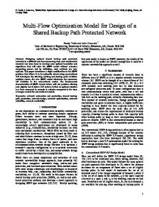
instances shown in Table 1. As a set of Pareto-optimal solutions is obtained in each simulation run, the minimum values of the solutions Z1 and Z2 are considered for comparison. For this purpose, each algorithm is employed 30 times to solve the five problem instances under different random environments shown in Table 2, each time considering a fixed optimum combination of the parameters obtained in the previous phase. The means of the 30 runs for each of the 5 problem instances solved by NSGA-II and NRGA are provided in Tables 6 and 7, respectively. Figure 5 shows the Pareto fronts of the solutions generated using NRGA and NSGA-II based on the fifth problem instance with the same input parameters of the supply chain.
28
NRGA *
NSGA-II *
Z2
Z2
Z1
Z1
Fig. 5: Pareto optimal fronts for the fifth problem instance by NRGA and NSGA-II algorithms
Table 6: The means of the six indicators resulted by NSGA-II Problem No. 1 2 3 4 5
135186.15 42135308.31 58760788.84 309611950.6 375029551.4
7554736.11 3770587537 3700114664 7810659933 1479493484
878025.76 7.2 3602784.13 165399400.2 10.8 1262227707 106113280 15.34 1022215667 213840106.7 11.46 1343676945 57461200.12 10.4 264159161
26.54 78.06 96.49 112.33 137.67
Table 7: The means of the six indicators resulted by NRGA Problem No. 1 2 3 4 5
131080.86 40509157.17 65153544.97 312147583.3 374143777
6829568.57 3662106158 3726733282 7759807997 1470280043
634660.99 8.14 2854693.44 152145873.1 13.06 1185415730 87151369.85 12.4 1104611819 207247695.1 12 1507231399 52741461.52 9.46 251050585
94.60 202.01 212.01 246.28 301.67
Two methods are used to compare the two algorithms; a two-sample t-test (Montgomery [28]) as well as one of MADM methods called simple additive weighting (SAW) (Hwang and Yoon [22]). In the first method, the results of the t-test on the means of problem for say are shown in Table 8. 29
obtained using the two algorithms on the first
Table 8: MSI mean comparison of employing the two algorithms in solving the first problem Levene's test for equality of the variances
F Equal variances assumed
Sig.
t-test for equality of the means
t
0.139 0.711 0.906
d.f.
P-value
Mean Difference
58
0.369
7.4809 105
95% confidence limits on the mean difference Std. Error of the Difference Lower Upper 8.2579 105
-9.0489 105
2.4014 106
Based on the results in Table 8, as the equality of the variances of the two samples cannot be rejected using the Levene's test, the two
means do not have a significant difference based on the t-statistic
obtained (the p-value of 0.369 is bigger than a usual significant level of 0.05 for say). Thus, the two algorithms have a similar
performance when they solve the first problem. The p-values of the other
measure comparisons in all problem instances are shown in Table 9. As seen in this table, there are only significant differences between the
means of the two algorithms obtained in all problem instances
(the p-values are shown with one star). This indicate that the results obtained using NSGA-II are validated using NRGA. Figures (6-11) show the comparisons between the means of the six measures better. Table 9: The p-values of the t-tests on the equality of the means of the six measures in all problem instances Problem No. 1 2 3 4 5
Z1 0.588 0.857 0.724 0.972 0.987
Z2 0.554 0.707 0.874 0.820 0.962
SI 0.239 0.670 0.200 0.894 0.262
NPI 0.379 0.270 0.586 0.621 0.270
MSI CPUTI 0.369 0.000* 0.309 0.000* 0.597 0.000* 0.433 0.000* 0.791 0.000*
* p-values less than 0.05 show significant differences
30
1E+10
400000000
8E+09
300000000
6E+09 NSGAII
200000000
NRGA
100000000
NSGAII
4E+09
NRGA
2E+09 0
0 1
2
3
4
1
5
Fig.6: Z1 mean comparison 20
200000000
15 NSGAII
100000000
3
4
5
Fig.7: Z2 mean comparison
250000000
150000000
2
NSGAII
10
NRGA
NRGA
5
50000000
0
0 1
2
3
4
1
5
Fig.8: SI mean comparison
2
3
4
5
Fig.9: NPI mean comparison 250
2E+09
200
1.5E+09
150
NSGAII
1E+09
NRGA
500000000
NSGAII
100
NRGA
50
0
0 1
2
3
4
5
1
Fig.10: MSI mean comparison
2
3
4
5
Fig.11: CPUTI mean comparison
In the second method, SAW is employed to determine which algorithm is preferable. As the SAW method starts with normalizing a decision matrix based on the linear method, a decision matrix is
first organized for m (here 2) alternatives and n indices (here 6) based on the desirability
of alternative i towards index j denoted by
. In the next step, an un-scaled weight matrix is made using 1/6 . Then, the total sum of each row
equal weights for each index ( 31
is computed. At the end, an algorithm with the largest total sum of weights (TSW) is selected for each of the problem instances. Table 10 shows TSWs of each algorithm in all problem instances. As seen in this table, NSGA-II is the better algorithm for all problem instances, while NRGA works satisfactorily. In short, based on the results obtained using the t-tests and the SAW method, it can be concluded that both algorithms work satisfactorily to optimize the SCN problem at hand. Table 10: Comparison results using the SAW method Problem No. 1 2 3 4 5
NSGA-II 0.9135 0.9466 0.9578 0.9682 0.9849
NRGA 0.8467 0.8876 0.8597 0.9080 0.8861
applicability NSGA-II NSGA-II NSGA-II NSGA-II NSGA-II
6. Conclusions and future studies In this paper, a novel mathematical formulation for a three-echelon supply chain network operating in an uncertain environment was developed. The problem was first formulated into a singleobjective stochastic mixed-integer linear model with chance-constraints. Then, it was reformulated to obtain a deterministic bi-objective mixed-integer nonlinear programming (MINLP). As the model developed in this study was hard to be solved analytically, a non-dominated sorting GA (NSGA-II) was utilized to find Pareto fronts. Since there was no benchmark available in the literature to validate the results obtained, another GA-based multi-objective evolutionary algorithm called non-dominated ranking genetic algorithm (NRGA) was used as well. In both algorithms, a modified priority-based three-section encoding was used. Besides, a heuristic method was proposed to decode the available encoding under a two-stage transportation model so that each algorithm give rise to Pareto fronts in a single simulation run. Five problem instances of small, medium, and large were used to demonstrate the application of the proposed methodology as well as to compare the performances in terms of the means of six performance measures. After the parameter calibration process of both algorithms based on a statistical method using 30 samples, the algorithms were employed to solve the problem instances, each 30 times. The results of t32
tests and the SAW method at the end showed that while both algorithms performed reasonably well in all problems, NSGA-II acted better than NRGA for all problem instances. There are several recommendations for future studies as follows: 1. Considering to use other meta-heuristics such as MOPSO, MOGA, multi-objective harmony search (MOHS) and multi-objective simulated annealing (MOSA) to solve the problem. Consequently, a comparison study can be made to compare the performances 2. Appling other mutation and crossover operators 3. Designing and analyzing the problem under a four-echelon SCN to maximize profit under budget constraint 4. Using other probability distributions such as the uniform distribution to model uncertainties involved. 4. Using queuing models to hybridize the problem further. 5. Considering some input parameters as fuzzy numbers. 6. Considering outsourcing to produce a proportion of the products in addition to in-house productions 7. Taking into account discounts or inflation for system costs 8. Designing the SCN using the De-Novo programming approach 9. Considering a distance parameter between the layers as well as travel times to transport the products to customer nodes
Acknowledgement The authors are thankful for constructive comments of the anonymous reviewers. Taking care of the comments certainly improved the presentation.
References [1]. Al Jadaan O, Rajamani L, Rao CR (2009). Non-dominated ranked genetic algorithm for solving constrained multi-objective optimization problems. Journal of Theoretical and Applied Information Technology 5: 714-725.
33
[2]. Al Jadaan O, Rao CR, Rajamani L (2006). Parametric Study to Enhance Genetic Algorithm Performance, Using Ranked based Roulette Wheel Selection method. InSciT, Merida, Spain, 274278. [3]. Altiparmak F, Gen M, Lin L, Paksoy T (2006). A genetic algorithm approach for multi-objective optimization of supply chain networks. Computers and Industrial Engineering 51: 196–215. [4]. Amiri A (2006). Designing a distribution network in a supply chain system: formulation and efficient solution procedure. European Journal of Operational Research 171: 567–576. [5]. Azaron A, Brown KN, Tarim SA, Modarres M (2008). A multi-objective stochastic programming approach for supply chain design considering risk. International Journal of Production Economics 116: 129–138. [6]. Bandyopadhyay S, Bhattacharya R (2014). Solving a tri-objective supply chain problem with modified NSGA-II algorithm. Journal of Manufacturing Systems 33: 41-50. [7]. Bidhandi HM, Yusuff b RM (2011). Integrated supply chain planning under uncertainty using an improved stochastic approach. Applied Mathematical Modeling 35: 2618–2630. [8]. Cardona-Valdés Y, Alvarez A, OzdemirD (2011). A bi-objective supply Alvarez chain design problem with uncertainty. Transportation Research Part C 19: 821–832. [9]. Cardona-Valdés Y, Alvarez A, Pacheco J (2014). Metaheuristic procedure for a bi-objective supply chain design problem with uncertainty. Transportation Research Part B: Methodological 60: 66-84. [10]. Chen C-L, Lee W-C (2004) Multi-objective optimization of multi-echelon supply chain networks with uncertain product demands and prices. Computers and Chemical Engineering 28: 1131–1144. [11]. Costa A, Celano G, Fichera, S, Trovato E (2010). A new efficient encoding/decoding procedure for the design of a supply chain network with genetic algorithms. Computers and Industrial Engineering 59: 986–999. [12]. Deb K, Pratap A, Agerwal S, Meyarivan T (2002). A fast and elitist multiobjective genetic algorithm: NSGA-II. IEEE Transactions on Evolutionary Computation 6: 182-197. [13]. El-Sayed M, Afia N, El-Kharbotly A (2010). A stochastic model for forward–reverse logistics network design under risk. Computers and Industrial Engineering 58: 423–431. [14]. Gebennini E, Gamberini R, Manzini R (2009). An integrated production–distribution model for the dynamic location and allocation problem with safety stock optimization. International Journal of Production Economics 122: 286–304. [15]. Gen M, Altiparmak F, Lin L (2006). A genetic algorithm for two-stage transportation problem using priority-based encoding. OR Spectrum 28: 337-354. [16]. Gen M, Cheng R (2000). Genetic algorithms and engineering optimization. New York: John Wiley and Sons. Gen M, Li YZ (1998). Solving multi-objective transportation problem by spanning tree[17]. base genetic algorithm. In: Adaptive computing in design and manufactured. Springer, Berlin Heidelberg New York, 98–108. [18]. Georgiadis MC, Tsiakis P, Longinidis P, Sofioglou MK (2011). Optimal design of supply chain networks under uncertain transient demand variations. Omega 39: 254-272. [19]. Guilléna G, Mele FD, Bagajewicz MJ, Espuna A, Puigjaner L (2005). Multi-objective supply chain design under uncertainty. Chemical Engineering Science 60: 1535 – 1553.
34
[20]. Hnaiena F, Delormeb X, Dolgui A (2010). Multi-objective optimization for inventory control in two-level assembly systems under uncertainty of lead times. Computers and Operations Research 37: 1835-1843. [21]. Hwang CL, Masud ASM (1979). Multiple-objective decision making, methods and applications: A state-of-the-art survey. Springer-Verlag, Berlin. [22]. Hwang CL, Yoon KL (1981). Multiple attribute decision making: methods and applications. Springer-Verlag, New York. [23]. Jamshidi R, Fatemi-Ghomi SMT, Karimi E (2012). Multi-objective green supply chain optimization with a new hybrid memetic algorithm using the Taguchi method. Scientia Iranica 19: 1876–1886. [24]. Marufuzzaman M, Eksioglu SD, Huang Y (2014). Two-stage stochastic programming supply chain model for biodiesel production via wastewater treatment. Computers & Operations Research 49:1-17. [25]. Mele FD, Guill´en G, Espuna A, Puigjaner L (2007). An agent-based approach for supply chain retrofitting under uncertainty. Computers and Chemical Engineering 31: 722–735. [26]. Mirzapour Al-e-hashem SMJ, Malekly H, Aryanezhad MB (2011). A multi-objective robust optimization model for multi-product multi-site aggregate production planning in a supply chain under uncertainty. International Journal of Production Economics 134: 28–42. [27]. Moncayo-Martı´nez LA, Zhang D Z ( 2011). Multi-objective ant colony optimization: A meta-heuristic approach to supply chain design. Int. J. Production Economics 131: 407–420. [28]. Montgomery CL (1995). Design and Analysis of Experiments. John Wiley & Sons Inc, New York. [29]. Murthy DNP, Solem BO, Roren T (2004). Product warranty logistics: issues and challenges. European Journal of Operational Research 156: 110-126. [30]. Olivares-Benitez E, González-Velarde JL, Ríos-Mercado RZ (2012). A supply chain design problem with facility location and bi-objective transportation choices. Sociedad de Estadística e Investigación Operativa 20: 729-753. [31]. Pishvaee MS, Razmi J, Torabi SA (2014). An accelerated Benders decomposition algorithm for sustainable supply chain network design under uncertainty: A case study of medical needle and syringe supply chain. Transportation Research Part E: Logistics and Transportation Review 67:14-38. [32]. Prakash A, Chan FTS, Liao H, Deshmukh SG (2012). Network optimization in supply chain: a KBGA approach. Decision Support Systems 52: 528–538. [33]. Rodriguez MA, Vecchietti AR, Harjunkoski L, Grossmann LE (2014). Optimal supply chain design and management over a multi-period horizon under demand uncertainty. Part I: MINLP and MILP models. Computers & Chemical Engineering 62:194-210. [34]. Ruiz-Femenia R, Guillén-Gosálbez G, Jiménez L, Caballero JA (2013). Multi-objective optimization of environmentally conscious chemical supply chains under demand uncertainty. Chemical Engineering Science 96: 1-11. [35]. Schüt PZ, Tomasgard A, Ahmed S (2009). Supply chain design under uncertainty using sample average approximation and dual decomposition. European Journal of Operational Research 199: 409–419.
35
[36]. Shankar BL, Basavarajappa S, Chen JCH, Kadadevaramath RS (2013). Location and allocation decisions for multi-echelon supply chain network – a multi-objective evolutionary approach. Expert Systems with Applications 40: 551–562. [37]. Shankar BL, Basavarajappa S, Kadadevaramath RS, Chen JCH (2013). A bi-objective optimization of supply chain design and distribution operations using non-dominated sorting algorithm: A case study. Expert Systems with Applications 40: 5730-5739. [38]. Snyder LV, (2006). Facility location under uncertainty: a review. IIE Transactions 38: 537–554. [39]. Song D-P, Dong j-x, Xu J (2014). Integrated inventory management and supplier base reduction in a supply chain with multiple uncertainties. European Journal of Operational Research 232(3):522-536. [40]. Sourirajan K, Ozsen L, Uzsoy R (2009). A genetic algorithm for a single product network design model with lead time and safety stock considerations. European Journal of Operational Research 197: 599–608. [41]. Tsai C-F, and Chao K-M (2009). Chromosome refinement for optimizing multiple supply chains. Information Sciences 179: 2403–2415. [42]. Van Landeghem, H, Vanmaele, H, (2002). Robust planning: a new paradigm for demand chain planning. Journal of Operation Management 20: 769–783. [43]. Wang H-F, Hsu H-W (2010). A closed-loop logistic model with a spanning-tree based genetic algorithm. Computers & Operations Research 37: 376-389. [44]. Wang K-J, Makond B, Liu S-Y (2011). Location and allocation decisions in a twoechelon supply chain with stochastic demand – a genetic-algorithm based solution. Expert Systems with Applications 38: 6125–6131. [45]. Wu D, Wu DD, Zhang Y, Olson DL (2013). Supply chain outsourcing risk using an integrated stochastic-fuzzy optimization approach. Information Sciences 235:242-258. [46]. You F, Grossmann IE (2008). Design of responsive supply chains under demand uncertainty. Computers and Chemical Engineering 32: 3090–3111. [47]. Zegordi SH, Abadi LNK, BeheshtiNia MA (2010). A novel genetic algorithm for solving production and transportation scheduling in a two-stage supply chain. Computers and Industrial Engineering 58: 373–381. [48]. Zhang G, Shang J, Li W (2011). Collaborative production planning of supply chain under price and demand uncertainty. European Journal of Operational Research 215: 590–603. [49]. Zitzler E, Thiele L (1999). Multi-objective evolutionary algorithms: A comparative case study and the strength Pareto approach. IEEE Transactions on Evolutionary Computation 3: 257– 271.
36