Computer Science and Engineering, Center for Evolutionary Medicine and Informatics, The Biodesign. Institute, Arizona State University, Tempe, AZ 85287.
A Multi-Task Learning Formulation for Predicting Disease Progression Jiayu Zhou, Lei Yuan, Jun Liu, Jieping Ye Computer Science and Engineering, Center for Evolutionary Medicine and Informatics, The Biodesign Institute, Arizona State University, Tempe, AZ 85287
{Jiayu.Zhou, Lei.Yuan, Jun.Liu, Jieping.Ye}@asu.edu ABSTRACT
General Terms
Alzheimer’s Disease (AD), the most common type of dementia, is a severe neurodegenerative disorder. Identifying markers that can track the progress of the disease has recently received increasing attentions in AD research. A definitive diagnosis of AD requires autopsy confirmation, thus many clinical/cognitive measures including Mini Mental State Examination (MMSE) and Alzheimer’s Disease Assessment Scale cognitive subscale (ADAS-Cog) have been designed to evaluate the cognitive status of the patients and used as important criteria for clinical diagnosis of probable AD. In this paper, we propose a multi-task learning formulation for predicting the disease progression measured by the cognitive scores and selecting markers predictive of the progression. Specifically, we formulate the prediction problem as a multi-task regression problem by considering the prediction at each time point as a task. We capture the intrinsic relatedness among different tasks by a temporal group Lasso regularizer. The regularizer consists of two components including an �2,1 -norm penalty on the regression weight vectors, which ensures that a small subset of features will be selected for the regression models at all time points, and a temporal smoothness term which ensures a small deviation between two regression models at successive time points. We have performed extensive evaluations using various types of data at the baseline from the Alzheimer’s Disease Neuroimaging Initiative (ADNI) database for predicting the future MMSE and ADAS-Cog scores. Our experimental studies demonstrate the effectiveness of the proposed algorithm for capturing the progression trend and the cross-sectional group differences of AD severity. Results also show that most markers selected by the proposed algorithm are consistent with findings from existing cross-sectional studies.
Algorithms
Keywords Alzheimer’s Disease, regression, multi-task learning, group Lasso, stability selection, cognitive score
1. INTRODUCTION Alzheimer’s disease (AD), the most common type of dementia, is characterized by the progressive impairment of neurons and their connections resulting in loss of cognitive function and ultimately death [20]. AD currently affects about 5.3 million individuals in United States and more than 30 million worldwide with a significant increase predicted in the near future [5]. Alzheimer’s disease has been not only the substantial financial burden to the health care system but also the psychological and emotional burden to patients and their families. As the research on developing promising new treatments to slow or prevent AD progressing, the need for markers that can track the progress of the disease and identify it early becomes increasingly urgent. A definitive diagnosis of AD can only be made through an analysis of brain tissue during a brain biopsy or autopsy [18]. Many clinical/cognitive measures have been designed to evaluate the cognitive status of the patients and used as important criteria for clinical diagnosis of probable AD, such as Mini Mental State Examination (MMSE) and Alzheimer’s Disease Assessment Scale cognitive subscale (ADAS-Cog) [25]. MMSE has been shown to be correlated with the underlying AD pathology and progressive deterioration of functional ability [18]. ADAS-Cog is the gold standard in AD drug trial for cognitive function assessment [31]. Since neurodegerenation of AD proceeds years before the onset of the disease and the therapeutic intervention is more effective in the early stage of the disease, there is thus an urgent need to address two major research questions: (1) how can we predict the progression of the disease measured by cognitive scores, e.g., MMSE and ADAS-Cog? (2) what is the smallest set of features (measurements) most predictive of the progression? The prime candidate markers for tracking disease progression include neuroimages such as magnetic resonance imaging (MRI), cerebrospinal fluid (CSF), and baseline clinical assessments [12]. The relationship between the cognitive scores and possible risk factors such as age, APOE gene, years of education and gender has been previously studied [36, 17]. Many existing works analyzed the relationship between cognitive scores and
Categories and Subject Descriptors H.2.8 [Database Management]: Database Applications— Data Mining; J.3 [Life and Medical Sciences]: Health, Medical information systems
Permission to make digital or hard copies of all or part of this work for personal or classroom use is granted without fee provided that copies are not made or distributed for profit or commercial advantage and that copies bear this notice and the full citation on the first page. To copy otherwise, to republish, to post on servers or to redistribute to lists, requires prior specific permission and/or a fee. KDD’11, August 21–24, 2011, San Diego, California, USA. Copyright 2011 ACM 978-1-4503-0813-7/11/08 ...$10.00.
814
temporal smoothness term, which ensures a small deviation between two regression models at successive time points. We have performed extensive experimental studies to evaluate the effectiveness of the proposed algorithm. We use various types of data from the Alzheimer’s Disease Neuroimaging Initiative (ADNI) database including MRI scans, CSF, and clinical scores at the baseline to predict the MMSE and ADAS-Cog scores for the next three years. Our experimental studies show that the proposed algorithm better captures the progression trend and the cross-sectional group differences of AD severity than existing methods. Results also show that most markers selected by the proposed algorithm are consistent with findings from existing crosssectional studies.
imaging markers based on MRI such as gray matter volumes, density and loss [3, 8, 15, 16, 33], shape of ventricles [14, 34] and hippocampal [34] by correlating these features with baseline MMSE scores. In [13], the intensity and volume of medial temporal lobe altogether with other risk factors and the gray matter were shown to be correlated with the 6month MMSE score, which allowed us to predict near-future clinical scores of patients. Relations between 6-month atrophy patterns in medial temporal region and memory declination in terms of clinical scores had also been examined in [27]. To predict the longitudinal response to Alzheimer’s Disease progression, Ashford and Schmitt built a model with horologic function using “time-index” to measure the rate of dementia progression [4]. In [10], the so-called SPARE-AD index was proposed based on spatial patterns of brain atrophy and its linear effect against MMSE was reported. In a more recent study by Ito et al., the progression rate of cognitive scores was modeled using power functions [17]. Most existing work employed either the regression model [13, 33] or the survival model [37] for modeling the disease progression. The correlation between the ground truth and the prediction is used to evaluate the model [13, 33]. When the size of covariates is small, each covariate can be individually added to the model to examine its effectiveness for predicting the target [17, 38], or univariate analysis is performed individually on all covariates and those who exceed a certain significance threshold are included in the model [27]. When the number of covariates is large and significant correlations among covariates exist, these approaches are suboptimal. To deal with the curse of dimensionality, dimension reduction techniques are commonly employed. Duchesne et al. used principle components analysis (PCA) to build a low dimensional feature space from image data [13]. An obvious disadvantage of dimension reduction techniques such as PCA is that the model is no longer interpretable, since all features are involved. Stonnington et al. used relevance vector regression (RVR), which integrated feature selection in the training stage [33]. These approaches only predict clinical scores at a single time point and their performances are far from satisfactory to be clinically useful for AD prognosis. In this paper, we propose a multi-task learning formulation for predicting the progression of the disease measured by the clinical scores at multiple time points and simultaneously selecting markers predictive of the progression. Specifically, we formulate the prediction of clinical scores at a sequence of time points as a multi-task regression problem, where each task concerns the prediction of a clinical score at one time point. Multi-task learning aims at improving the generalization performance by learning multiple related tasks simultaneously. The key of multi-task learning is to exploit the intrinsic relatedness among the tasks. For the disease progression considered in this paper, it is reasonable to assume that a small subset of features is predictive of the progression, and the multiple regression models from different time points satisfy the smoothness property, that is, the difference of the cognitive scores between two successive time points is small. To this end, we develop a novel multitask learning formulation based on a temporal group Lasso regularizer. The regularizer consists of two components including an �2,1 -norm penalty [39] on the regression weight vectors, which ensures that a small subset of features will be selected for the regression models at all time points, and a
2. PROPOSED MULTI-TASK REGRESSION FORMULATION In the longitudinal AD study, we measure the cognitive scores of selected patients repeatedly at multiple time points. By considering the prediction of cognitive scores at a single time point as a regression task, we formulate the progression of clinical scores as a multi-task regression problem. We employ the multi-task regression formulation instead of solving a set of independent regression problems since the intrinsic temporal smoothness information among different tasks can be incorporated into the model as prior knowledge. Consider a multi-task regression problem of t time points with n training samples of d features. Let {x1 , x2 , · · · , xn } be the input data at the baseline, and {y1 , y2 , · · · , yn } be the targets, where each xi ∈ Rd represents a sample (patient), and yi ∈ Rt is the corresponding targets (clinical scores) at different time points. In this paper we employ linear models for the prediction. Specifically, the prediction model for the ith time point is given by f i (x) = xT wi , where wi is the weight vector of the model. Let X = [x1 , · · · , xn ]T ∈ Rn×d be the data matrix, Y� = [y1 , · · · , y�n ]T ∈ Rn×t be the target matrix, and W = w1 , w2 , ..., wt ∈ Rd×t be the weight matrix. One simple approach is to estimate W by minimizing the following objective function: min �XW − Y �2F + θ1 �W �2F , W
(1)
where the first term measures the empirical error on the training data, the second (penalty) term controls the generalization error, θ1 > 0 is a regularization parameter, and �.�F is the Frobenius norm of a matrix. The regression method above is known as the ridge regression and it admits an analytical solution given by: W = (X T X + θ1 I)−1 X T Y.
(2)
One major limitation of the regression model above is that the tasks at different time points are assumed to be independent with each other, which is not the case in the longitudinal AD study considered in this paper.
2.1 Temporal Smoothness Prior To capture the temporal smoothness of the cognitive scores at different time points, we introduce a regularization term in the regression model that penalizes large deviations of predictions at neighboring time points, resulting in the fol-
815
Let S i be the ith column of S. We therefore denote X(i) = PS i (X) ∈ Rni ×d as the input data matrix of the ith task, and y(i) = PS i (Y i ) ∈ Rni ×1 as the corresponding target vector, where ni is number of samples from the ith task. Similar to the case without missing target values considered in Section 2.1, we take the derivative of Eq.(10) with respect to wi (2 ≤ i ≤ t − 1) and set it to zero:
lowing formulation: min �XW − Y �2F + θ1 �W �2F + θ2 W
t−1 � �2 � � i i+1 � �w − w � , (3) 2
i=1
where θ2 ≥ 0 is a regularization parameter controlling the temporal smoothness. This temporal smoothness term can be expressed as:
Awi−1 + Mi wi + Awi+1 = Ti ,
t−1 � �2 � � i i+1 � 2 �w − w � = �W H�F ,
where A, Mi , and Ti are defined as follows:
F
i=1
A = −θ2 Id ,
where H ∈ Rt×(t−1) is defined as follows: Hij = 1 if i = j, Hij = −1 if i = j + 1, and Hij = 0 otherwise. The formulation in Eq.(3) becomes: min �XW − Y W
�2F
+
θ1 �W �2F
+
θ2 �W H�2F
.
T Mi = X(i) X(i) + θ1 Id + 2θ2 Id , T y(i) . Ti = X(i)
� �2 For the special case i = 1, the term �wi−1 − wi �2 does not � �2 exist, nor is the term �wi − wi+1 �2 for i = t. We combine the equations for all tasks (1 ≤ i ≤ t), which can be represented as a block tridiagonal linear system: ⎛ ⎞⎛ 1 ⎞ ⎛ ⎞ w M1 A T1 0 ⎜ A M2 A ⎟ ⎜ w 2 ⎟ ⎜ T2 ⎟ ⎜ ⎟⎜ ⎟ ⎜ ⎟ ⎜ ⎟⎜ . ⎟ ⎜ . ⎟ .. ⎜ ⎟ ⎜ .. ⎟ = ⎜ .. ⎟ (12) . ⎜ ⎟⎜ ⎟ ⎜ ⎟ ⎝ A Mt−1 A ⎠ ⎝wt−1 ⎠ ⎝Tt−1 ⎠ 0 A Mt Tt wt
(4)
The optimization problem in Eq.(4) admits an analytical solution, as shown below. First, we take the derivative of Eq.(4) with respect to W and set it to zero: X T XW − X T Y + θ1 W + θ2 W HH T � � � � X T X + θ1 Id W + W θ2 HH T
= 0,
(5) T
= X Y,
(6)
where Id is the identity matrix of size d by d. Since both matrices (X T X +θ1 Id ) and θ2 HH T are symmetric, we write the eigen-decomposition of these two matrices by Q1 Λ1 QT1 and (1) (2) (d) Q2 Λ2 QT2 , where Λ1 = diag(λ1 , λ1 , . . . , λ1 ) and Λ2 = (1) (2) (d) diag(λ2 , λ2 , . . . , λ2 ), are their eigenvalues, and Q1 and Q2 are orthogonal. Plugging them into Eq. (6) we get: Q1 Λ1 QT1 W + W Q2 Λ2 QT2 Λ1 QT1 W Q2
+
QT1 W Q2 Λ2
=
X T Y,
=
QT1 X T Y
For a general linear system of size td, it can be solved using Gaussian elimination with a time complexity of O((td)3 ). For our block tridiagonal system, the complexity is reduced to O(d3 t) using block Gaussian elimination. For large-scale linear systems, the LSQR algorithm [30], a popular iterative method for the solution of large linear systems of equations, can be employed with a time complexity of O(N td2 ), where N , the number of iterations, is typically small.
(7) Q2 .
(8)
ˆ = QT1 W Q2 and D = QT1 X T Y Q2 . Eq.(8) beDenote W ˆ +W ˆ Λ2 = D. Thus W ˆ is given by: comes Λ1 W ˆ i,j = W
Di,j (i)
(j)
.
2.3 Temporal Group Lasso Regularization Because of the limited availability of subjects in the longitudinal AD study and a relatively large number of features at ADNI including MRI features, the prediction model suffers from the so called “curse of dimensionality”. In addition, many patients drop out from the longitudinal study after a certain period of time, which reduces the effective number of samples. One effective approach is to reduce the dimensionality of the data. However, traditional dimension reduction techniques such as PCA are not desirable since the resulting model is not interpretable, and traditional feature selection algorithms are not suitable for multi-task regression with missing target values. In the proposed formulation, we employ the group Lasso regularization based on the �2,1 -norm penalty for feature selection [39], which assumes that a small set of features are predictive of the progression. The group Lasso regularization ensures that all regression models at different time points share a common set of features. Together with the temporal smoothness penalty, we obtain the following formulation:
(9)
λ1 + λ2
ˆ QT2 . The optimal weight matrix is then given by W ∗ = Q1 W
2.2 Dealing with Incomplete Data The clinical scores for many patients are missing at some time points, i.e., the target vector yi ∈ Rt may not be complete. A simple strategy is to remove all patients with missing target values, which, however, significantly reduces the number of samples. We consider to extend the formulation in Eq.(4) with missing target values in the training process. In this case, the analytical solution to Eq.(4) no longer exists. We show how the algorithm above can be adapted to deal with missing target values. We use a matrix S ∈ Rn×t to indicate missing target values, where Si,j = 0 if the target value of sample i is missing at the jth time point, and Si,j = 1 otherwise. We use the componentwise operator � as follows: Z = A � B denotes zi,j = ai,j bi,j , for all i, j. The formulation in Eq.(4) can be extended to the case with missing target values as: min �S � (XW − Y )�2F + θ1 �W �2F + θ2 �W H�2F . W
(11)
min �S�(XW − Y )�2F +θ1�W �2F +θ2�W H�2F +δ�W �2,1 (13) W �� � t 2 where �W �2,1 = di=1 j=1 Wij , and δ is a regularization parameter. When there is only one task, i.e., t = 1, the above formulation reduces to Lasso [35]. When t > 1, the weights of one feature over all tasks are grouped using the
(10)
Denote Pr (.) as the row selection operator parameterized by a selection vector r. The resulting matrix of Pr (A) includes only Ai such that ri �= 0, where Ai is the ith row of A.
816
tion [42], multiple thresholding procedures [41], or multistage methods [23, 40]. In this paper, we employ a standard two-stage procedure. In the first stage the algorithm selects features using longitudinal stability selection, resulting in a ˆ stable . In the second stage the algorithm subset of features U performs temporal smoothness regularized regression using selected features. We summarize the proposed algorithm in Algorithm 1.
�2 -norm, and all features are further grouped using the �1 norm. Thus, the �2,1 -norm penalty tends to select features based on the strength of the feature over all t tasks. The objective in Eq.(13) can be considered as a combination of a smooth term and a non-smooth term. The gradient descent or accelerated gradient method (AGM) [29, 28] can be applied to solve the optimization. One of the key steps in AGM is the computation of the proximal operator associated with the �2,1 -norm regularization. We employ the algorithm in the SLEP package [22], which computes the proximal operator associated with the general �1 /�q -norm efficiently.
Algorithm 1 Temporal Group Lasso Multi-Task Regression (TGL) Input: S, X, Y, θ1 , θ2 Δ, γ, η ˆ stable Output: W ∗ , U 1: Stage 1: longitudinal stability selection 2: Set K = {the feature set in X} 3: for δ ∈ Δ do 4: for j = 1 to γ do X Y 5: Subsample B(j) = {B(j) , B(j) } from {X, Y } (j) ˜ 6: Compute W by solving Eq.(13) with δ, B(j) ˜ (j) �= 0} 7: Set U δ (B(j) ) = {k : W 8: end for ˆ δk = �γ I(k ∈ U δ (B(j) ))/γ, ∀k ∈ K 9: Calculate Π j=1 10: end for ˆ δk ), ∀k ∈ K 11: Calculate S(k) = maxδ∈Δ (Π stable ˆ = {k: S(k) ranks among top η in K} 12: Set U 13: Stage 2: temporal smoothness regularized regression ˆ = X restricted to the features from U ˆ stable 14: Set X 15: if ∃p, q such that Sp,q = 0 then ˆ stable |, A = −θ2 Id 16: Set t = number of tasks, d = |U 17: for i = 1 to t do ˆ y(i) = PSi (Y i ) 18: X(i) = PSi (X), T T y(i) 19: Mi = X(i) X(i) + θ1 Id + 2θ2 Id , Ti = X(i) 20: end for 21: Obtain W ∗ by solving Eq.(12) with {Mi }, {Ti }. 22: else 23: Compute the analytical solution W ∗ as in Section 2.1. 24: end if
2.3.1 Longitudinal Stability Selection An important issue in the practical application of the proposed formulation is the selection of an appropriate amount of regularization, known as model selection. Cross validation is commonly used for model selection, however it tends to select more features than needed [26]. In this paper, we adapt stability selection to perform model selection for the proposed multi-task regression. Stability selection is a method recently proposed to address the problem of proper regularization using subsampling/bootstrapping [26]. It should be noted that in our formulation we find in our experiments that the list of top features selected by stability selection is not sensitive to the regularization parameters θ1 and θ2 . We thus focus on the selection of δ, which controls the sparsity of the model, in stability selection. Let K be the index set of features, i.e., k ∈ K denotes a feature. Given a set of regularization parameter values Δ and an iteration number γ, longitudinal stability selection X Y works as follows. Let B(j) = {B(j) , B(j) } be a random subsample from {X, Y } of size �n/2 without replacement. For ˜ (j) be the optimal solution of Eq.(13) on a given δ > 0, let W ˜ (j) �= 0} as the set of feaB(j) . Denote U δ (B(j) ) = {k : W k ˜ (j) . This process is repeated tures selected by the model W ˆ δk of each feature k for γ times � and selection probability Π γ δ is given by j=1 I(k ∈ U (B(j) ))/γ, where I(.) is the indicator function defined as follows: I(c) = 1 if c is true and ˆ δk computes the fraction I(c) = 0 otherwise. It is clear that Π of bootstrap experiments for which the feature k is selected. Repeat the above procedure for all δ ∈ Δ, and we define the ˆ δk ). stability score for each feature k by S(k) = maxδ∈Δ (Π stable ˆ we can To find a suitable size of stable feature set U either use top η stable features: ˆ stable
U
3. EXPERIMENTS In this section we evaluate the proposed algorithm on the ADNI database1 . The source codes are available online [1].
3.1 Experimental Setup In the ADNI project, MRI scans, CSF measurements, and clinical scores from selected patients are obtained repeatedly over a 6-month or 1-year interval. We denote each time point by the duration starting from the baseline when the patient came to the hospital for screening. For instance, M06 indicates 6 months after the baseline. We use different combinations of MRI (M), CSF (C), and META (M) (see Table 1) at baseline to predict MMSE and ADAS-Cog scores at four time points: M06, M12, M24, and M36. For MRI, we download 1.5T MRI data of 675 patients preprocessed by UCSF using FreeSurfer. MRI features can be grouped into 5 categories: cortical thickness average (CTA), cortical thickness standard deviation (CTStd), volume of cortical parcellation (Vol. Cort.), volume of white matter parcellation (Vol. WM.), and surface area (Surf. A.). There are 313 MRI features in total. We remove all samples which fail the MRI quality controls. For other feature
= {k : S(k) ranks among top η in K},
or use threshold πthr on the stability score: ˆ stable = {k : S(k) ≥ πthr }. U In our application we choose the top η features. Indeed, cross validation can be performed to determine how many features are needed. However, our empirical results show that using top η = 20 features is sufficient in most cases of our application.
2.4 Proposed Algorithm One undesired property of sparse learning methods such as Lasso is that the coefficients corresponding to relevant features are shrunk towards zero [40]. This shrinkage effect would lead to sub-optimal performance. To resolve this problem, existing methods apply adaptive regulariza-
1
817
www.loni.ucla.edu/ADNI/
significantly outperforms ridge regression. This is especially the case when the feature space is large and the sample size is small, e.g., CM and CEM (see Table 2). Note that multitask learning effectively increases the number of samples by learning multiple related tasks simultaneously, while ridge regression treats all tasks independently. Our results verify the effectiveness of multi-task learning for disease progression. Table 3: Comparison of our proposed approach (TGL) and ridge regression (RidR) on longitudinal MMSE prediction using different data combinations measured by R-value and average P-value. Performance at each time point is reported in terms of Rvalue. Weighted averages of R-values and P-values across all time points are also given.
Table 1: Features included in the META dataset. Note that the cognitive scores at the baseline are used to predict the future cognitive scores. A detailed explanation of each cognitive score and lab test can be found at [1]. Type Demographic Genetic Cognitive scores
Lab tests
Details age, yrs. of education, gender ApoE-ε4 information MMSE, ADAS-Cog, ADAS-MOD, ADAS subscores, CDR, FAQ, GDS, Hachinski, Neuropsychological Battery, WMS-R Logical Memory RCT1, RCT11, RCT12, RCT13, RCT14, RCT1407, RCT1408, RCT183, RCT19, RCT20, RCT29, RCT3, RCT392, RCT4, RCT5, RCT6, RCT8
sets, we remove samples with missing entries. Each feature combination includes the intersection of available samples, that is the combined dataset has no missing values. Because changes of MMSE and ADAS-Cog are both found to be closely correlated with the baseline MMSE score [17], we include the baseline MMSE score in all feature combinations. With the pre-processing procedure described above, the number of samples available for MMSE and ADAS-Cog at different time points are described in Table 2.
C E CE M EM CM
Table 2: The first column of the table indicates the different combinations of three datasets. The numbers of samples for different combinations available for both MMSE and ADAS-Cog at different time points are shown in the table together with the data dimensionality (Dim). C, E, and M refer to CSF, META, and MRI, respectively.
CEM
TGL RidR TGL RidR TGL RidR TGL RidR TGL RidR TGL RidR TGL RidR
M06 0.74 0.74 0.83 0.82 0.80 0.77 0.77 0.68 0.83 0.71 0.73 0.25 0.80 0.29
M12 0.72 0.72 0.84 0.83 0.82 0.80 0.75 0.67 0.84 0.71 0.73 0.34 0.83 0.36
M24 0.71 0.71 0.84 0.84 0.82 0.79 0.77 0.71 0.85 0.74 0.76 0.36 0.83 0.59
M36 0.65 0.65 0.78 0.76 0.72 0.71 0.70 0.63 0.80 0.54 0.69 0.48 0.72 0.56
AvgR 0.71 0.71 0.82 0.82 0.80 0.77 0.75 0.68 0.83 0.69 0.73 0.35 0.80 0.43
P-Val 3.3e-026 3.3e-026 7.4e-080 2.8e-075 7.2e-034 7.8e-033 2.7e-059 1.2e-045 3.8e-088 7.1e-032 1.3e-030 1.0e-006 8.4e-034 2.4e-008
Table 4: Comparison of our proposed approach (TGL) and ridge regression (RidR) on longitudinal ADAS-Cog prediction using different data combinations measured by R-value and average P-value.
MMSE ADAS-Cog Dim M06 M12 M24 M36 M06 M12 M24 M36 C 332 331 295 198 332 328 294 194 6 E 648 641 567 387 646 636 563 377 52 CE 332 331 295 198 332 328 294 194 57 M 648 641 567 387 646 636 563 377 306 EM 648 641 567 387 646 636 563 377 357 CM 332 331 295 198 332 328 294 194 311 CEM 332 331 295 198 332 328 294 194 362
C E CE M
3.2 Prediction Performance
EM
In this experiment, we compare our proposed approach with ridge regression on the prediction of MMSE and ADASCog using various types of data combinations. We report the results based on the leave-one-out scheme due to the small sample size. 5-fold cross validation is used to select model parameters (θ1 , θ2 in our approach and θ1 in ridge regression) in the training data (between 10−3 and 103 ). To compare with related works [33, 13], we use correlation coefficient (R-value) given by the correlation between the predicted values and the ground truth, and its correlation significance (P-value) as the evaluation criteria. P-value is given by testing the hypothesis of no correlation [2]. A good prediction model has a high R-value and low P-value (less than 0.0001 for example). The overall performance of the prediction is averaged across all time points weighted by the sample size. The results for MMSE and ADAS-Cog are summarized in Tables 3 and 4, respectively. Overall, the proposed approach
CM CEM
TGL RidR TGL RidR TGL RidR TGL RidR TGL RidR TGL RidR TGL RidR
M06 0.70 0.70 0.87 0.87 0.86 0.86 0.75 0.66 0.87 0.80 0.75 0.55 0.87 0.69
M12 0.71 0.71 0.87 0.86 0.85 0.84 0.78 0.71 0.87 0.81 0.77 0.60 0.86 0.66
M24 0.71 0.70 0.86 0.86 0.86 0.85 0.76 0.67 0.86 0.80 0.75 0.62 0.87 0.63
M36 0.66 0.66 0.83 0.83 0.80 0.74 0.74 0.61 0.84 0.70 0.74 0.53 0.81 0.40
AvgR 0.70 0.70 0.86 0.86 0.85 0.83 0.76 0.67 0.86 0.79 0.76 0.58 0.86 0.62
P-Val 1.7e-026 1.5e-026 2.6e-099 4.1e-097 1.7e-044 2.7e-035 4.4e-066 4.9e-041 3.2e-104 2.4e-058 2.5e-035 5.4e-016 1.9e-046 8.6e-010
In Table 5 we compare our approach with three closely related works. In [13], PCA was employed to reduce the dimensionality of the MRI data. Since only limited samples were used, the proposed method resulted in low prediction performance. To the best of our knowledge, the work in [13] is the only one that tried to predict cognitive scores at future time points and reported R/P-Value for comparison. The other two works used the ADNI database as in our study. Stonnington’s work predicted baseline cognitive scores using relevance vector regression (RVR) which enforced sparsity in the model [33]. Their regression results were better than those reported in [13]. However their prediction performance is much lower than ours. This is possibly due
818
to the use of different prediction models. Specifically, the model in [33] did not utilize rich temporal smoothness information as in the proposed approach. In [17], very limited risk factors were manually included and tested in their progression model. No actual prediction on the test data was performed. Instead, a visual comparison of the proposed model for different groups was provided, which was similar to our cross-sectional analysis in Section 3.3. It is hard to directly compare their approach with ours, since no prediction measures were reported in [17].
Ridge Regression Group [ ALL ]
Our Approach Group [ ALL ]
Ground Truth Group [ ALL ]
Group [ AD ]
Group [ AD ]
Group [ AD ]
Group [ MCI ]
Group [ MCI ]
Group [ MCI ]
Group [ NL ]
Group [ NL ]
Group [ NL ]
30 20 10
30 20 10
3.3 Cross-Sectional Progression 30
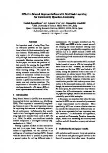
In this experiment, we study the cross-sectional progression patterns. We predict the progression of different patient groups using models built by ridge regression and our proposed approach on the CEM dataset. The predicted progressions for different groups including AD, MCI, and NL2 are visualized in a cross-sectional fashion with the mean values of prediction by different methods and the group truth provided. The results are summarized in Figure 1 and Figure 2. For MMSE, the target progression in probable AD patients shows a significant declination pattern, with an annual declination of 3.167 ± 0.40. For MCI patients we observe a slight annual declination of 0.919 ± 0.188. For normal controls, the MMSE scores are very stable with an annual declination of 0.032 ± 0.025. A similar pattern can be observed for ADAS-Cog. Probable AD patients have an annual growth on ADAS-Cog of 7.066 ± 2.257, while for the MCI group the annual growth is 1.558 ± 0.401. In normal controls, we observe a very small annual change (0.007 ± 0.565). We can also observe from Figure 1 and Figure 2 that the proposed approach can better capture the characteristics of the disease progression measured by clinical scores for different groups of patients. The proposed method performs significantly better than ridge regression for the probable AD group and the MCI group at M36 where the number of training samples is small. The result further verifies the effectiveness of multi-task learning for disease progression especially for small sample size problems.
20 10
30 20 10 M6 M12
M24
M36
M6 M12
M24
M36
M6 M12
M24
M36
Figure 1: Visual predictive comparison for MMSE on the CEM dataset. The first, second, third, and fourth rows show the results for the complete dataset (ALL), the AD group (AD), the MCI group (MCI), and the NL group (NL), respectively. The left column shows ridge regression results. The middle column shows the results using our proposed approach. The ground truth values are plotted in the right column. The red line connects the mean values of each time point.
vious studies [9, 19, 3]. Besides hippocampus and middle temporal, we also find isthmus cingulate a very stable feature for MMSE. The atrophy of isthmus cingulate is considered high in AD patients [24]. In addition, CTA of left inferior parietal and volume of right inferior parietal are also found to be stable. This agrees with evidence from the previous study that includes pathological confirmation of the diagnosis [21], which shows that parietal atrophy contributes to predictive values for diagnosing AD. To access the effectiveness of CSF features, we perform longitudinal stability selection on the data combining CSF and MRI (Figure 4). In CSF, we use 3 simple features (Aβ42, t-tau and p-tau) and 2 ratio features (t-tau/Aβ-42 and p-tau/Aβ-42). We observe that Aβ-42 and p-tau are among the top three markers, whereas t-tau is not selected in both targets. Figure 5 shows the stability results of META features (see Table 1). Baseline clinical test scores (MMSE, ADAS-MOD, ADAS-Cog, ADAS-Cog subscores, CDR) and neuropsychological test scores (TRAASCORE, GATVEGESC) are found to be important features for both scores. Among ADAS-Cog subscores, Word Recall (subscore 1) and Orientation (subscore 7) are found to be important. These findings agree with recent itemized ADAS-Cog analysis, where orientation was found to be the most sensitive item in cross-sectional study of cognitive impairment [32]. The results of stability selection after adding META to MRI are shown in Figure 6. Many MRI features have low stability scores. A possible explanation is that some clinical tests included in META
3.4 Feature Evaluation In this experiment we evaluate the relevance of features selected by longitudinal stability selection on different feature combinations. Given the range of regularization parameter values Δ, the set of selected features is a function of input data X and target Y , thus for the same data set X but different targets (clinical scores) Y , the algorithm may select different features. Indeed, although different clinical scores are used to measure the cognition status, they may emphasize different aspects of the AD pathology. The top MRI markers selected by longitudinal stability selection are shown in Figure 3. We observe that volume of left hippocampus, CTA of middle temporal gyri and CTA of left and right entorhinal are among the most stable features for both MMSE and ADAS-Cog scores. These findings agree with the known knowledge that in the pathological pathway of AD, medial temporal lobe (hippocampus and entorhinal cortex) is firstly affected, followed by progressive neocortical damage [7, 11]. Evidence of a significant atrophy of middle temporal gyri in AD patients has also been observed in pre2 AD, MCI, and NL refer to Alzheimer’s Disease patients, Mild Cognitive Impairment patients, and normal controls, respectively.
819
Table 5: Comparison of the proposed approach with three related works in the literature. AD, MCI, and NL refer to Alzheimer’s Disease patients, Mild Cognitive Impairment patients, and normal controls, respectively. Method Duchesne et al. [13]
Target M06 MMSE
Subjects 75 NL, 49 MCI, 75 AD
Stonnington et al. [33]
baseline MMSE and ADAS-Cog M06-M36 ADAS-Cog
Set1: 73 AD, 91 NL Set2 (ADNI): 113 AD, 351 MCI, 122 NL ADNI: 186 AD, 402 MCI, 229 NL
M06-M36 MMSE and ADAS-Cog
ADNI: 133 AD, 304 MCI, 188 NL
Ito et al. [17]
Our approach
Ridge Regression Group [ ALL ]
Our Approach Group [ ALL ]
Feature Baseline MRI, age, gender, years of education Baseline MRI, CSF
Age, APOE4, gender, family history, years of education Baseline MRI, CSF, and META (see Table 1 for details)
1
Ground Truth Group [ ALL ]
Result MMSE: 0.31 (p=0.03)
MMSE: Set1: 0.7 (p