J. Parallel Distrib. Comput. 73 (2013) 293–302
Contents lists available at SciVerse ScienceDirect
J. Parallel Distrib. Comput. journal homepage: www.elsevier.com/locate/jpdc
Parallel multitask cross validation for Support Vector Machine using GPU Qi Li ∗ , Raied Salman, Erik Test, Robert Strack, Vojislav Kecman Virginia Commonwealth University, Richmond, VA, 23220, United States
article
info
Article history: Received 27 April 2011 Received in revised form 16 January 2012 Accepted 19 February 2012 Available online 26 February 2012 Keywords: Support Vector Machine Cross validation GPU Parallel computing
abstract The Support Vector Machine (SVM) is an efficient tool in machine learning with high accuracy performance. However, in order to achieve the highest accuracy performance, n-fold cross validation is commonly used to identify the best hyperparameters for SVM. This becomes a weak point of SVM due to the extremely long training time for various hyperparameters of different kernel functions. In this paper, a novel parallel SVM training implementation is proposed to accelerate the cross validation procedure by running multiple training tasks simultaneously on a Graphics Processing Unit (GPU). All of these tasks with different hyperparameters share the same cache memory which stores the kernel matrix of the support vectors. Therefore, this heavily reduces redundant computations of kernel values across different training tasks. Considering that the computations of kernel values are the most time consuming operations in SVM training, the total time cost of the cross validation procedure decreases significantly. The experimental tests indicate that the time cost for the multitask cross validation training is very close to the time cost of the slowest task trained alone. Comparison tests have shown that the proposed method is 10 to 100 times faster compared to the state of the art LIBSVM tool. © 2012 Elsevier Inc. All rights reserved.
1. Introduction The recent developments of Graphics Processing Unit (GPU) have shown superb computational performance on floating point operations compared to the current multi-core CPU. Certain high performance GPUs are now designed to solve general purpose computing problems instead of graphics rendering, which was considered as the sole purpose of using GPUs previously. Many research work have shown promising performance results gained by using GPUs on a wide area of topics. The speed performance of Support Vector Machine (SVM) has been improved by using GPU through both the training and testing phases shown in [1]. Although not all algorithms can be parallelized, some applications can benefit from the massive parallel processing capability of GPU by doing some very simple tweaks such as using GPU Basic Linear Algebra Subroutines (CUBLAS) [18]. Most of these algorithms are often called data parallel algorithms [13]. Task level parallelism is not the primary advantage of GPU compared to multi-core CPU, however possibilities of using both task and data level parallelism should be explored and analyzed in order to achieve the maximum performance of GPU. This is our starting point of developing the parallel SVM algorithm and its cross validation procedure using GPU. Support Vector Machine [23] is a learning algorithm which has become popular due to its high accuracy performance in solving
∗
Corresponding author. E-mail addresses:
[email protected],
[email protected] (Q. Li).
0743-7315/$ – see front matter © 2012 Elsevier Inc. All rights reserved. doi:10.1016/j.jpdc.2012.02.011
both regression and classification tasks. Nevertheless, the training phase of an SVM is a computationally expensive task because the core part of the training stage is solving a QP problem [20]. There are countless efforts and studies which have been done on how to reduce the training time of SVM. After Vapnik invented SVM, he described a method known as ‘‘chunking’’ to break down the large QP problem into a series of smaller QP problems. This method significantly reduced the size of the matrix but it still could not solve large problem due to the computer memory limitations at that time. Osuna et al. presented a decomposition approach using iterative methods in [19]. Joachims introduced practical techniques such as shrinking and kernel caching in [16], which are common implementation in many modern SVM softwares today. He also published his own SVM software called SVMLight [16] that uses these techniques. Platt invented SMO [20] to solve the standard QP problem by iteratively solving a QP problem with only two unknowns using analytical methods. This method requires a small amount of computer memory. Therefore, it addresses the memory limitation issue brought by large training data sets. Later on, Keerthi et al. developed an improved SMO in [17], which resolved the slow convergence issue in Platt’s method. More recently Fan et al. introduced a series of working set selection [9], which further improved the speed of convergence. The method has been implemented in the state of the art LIBSVM software [5]. Huang et al. developed the ISDA algorithm [14] to solve the SVM QP problem without the bias. The above major contributions summarize the work of how to implement a fast classic SVM in sequential programming.
294
Q. Li et al. / J. Parallel Distrib. Comput. 73 (2013) 293–302
Some earlier works using parallel techniques in SVM can be found in [6,8,24,15]. Cao et al. presented a very practical Parallel SMO [3] implemented with Message Passing Interface on a cluster system. The performance gain of training SVM using clusters shows the beauty of parallel processing. This method is also the foundation of the proposed GPUSVM. Graf et al. introduced the Cascade SVM [11] which decomposes the training data set to multiple chunks and trains them separately. Then the support vectors from different individual classifiers are combined and fed back to the system again. They proved that the global optimal solution can be achieved by using this method. This parallelism is in the task level compared to the data level parallelism in Cao et al.’s work [3]. Cascade SVM offers a way to handle ultra-large data set training. Catanzaro et al. proposed a method to train a binary SVM classifier using GPU in [4]. Significant speed improvement is reported compared to the LIBSVM software. The latest GPU version of SVM is from [12]. They enable the possibility of training a multiclass classification problem on a GPU. Cross validation [22,2] is a commonly used procedure which searches for the best hyperparameters. Particularly, n-fold cross validation is generally used for SVM training. Most current SVM tools offer cross validation function by sequentially training through a group of different hyperparameter combinations. These tasks usually run one by one and do not communicate with each other. People tend to use multi-threading to run multiple tasks at the same time but they are still independent from each other. And the performance gain of multi-threading highly depends upon the hardware specification. Our aim is letting the multiple training tasks be aware of each other and share the kernel matrix cached in memory. The novelty of this method let every task synchronize together at each iteration of the training phase and if some of these tasks share the same support vectors, there is no need to do duplicated kernel computations but simply fetch the kernel results from the memory. The most time consuming part, which is the nonlinear kernel computations, can be heavily reduced. This paper is organized as follows. Section 2 briefly reviews the basic principles of SVM. Section 3 introduces the GPU hardware and its software platform CUDA for general purpose computing. Section 4 explains the parallel SMO algorithm implemented on GPU and the implementation for cross validation procedure. Performance results of the proposed algorithm are presented and analyzed in Section 5. Section 6 summarizes the conclusions and points out the future research direction.
2.1. Linear SVM with L1 soft margin
min
w, ⃗ b,ζ⃗
2
||w|| ⃗ +C
α⃗
2 i =1 j =1
s.t. ∀i : 0 ≤ αi ≤ C
and
(⃗ ⃗ )αi αj −
yi yj xTi xj
n
αi ,
(2)
i =1
n
yi αi = 0.
i=1
The Lagrangian multiplier αi has a box constraint and an equality constraint shown in Eq. (2). And each data point ⃗ xi is associated with one αi . In order to guarantee the existence of an optimal point for a positive definite QP problem, the Karush–Kuhn–Tucker (KKT) conditions should be satisfied. The KKT conditions for the QP problem described in Eq. (2) are met when
∀i : αi (yi d(⃗xi ) − 1 + ζi ) = 0, (C − αi )ζi = 0, αi ≥ 0 and ζi ≥ 0.
(3)
d(⃗ xi ) is the predicted output label. There are three different cases for αi : 1. αi = 0. Then ζi = 0. Thus ⃗ xi is correctly classified. 2. 0 < αi < C . Then yi d(⃗ xi ) − 1 + ζi = 0 and ζi = 0. Therefore, yi d(⃗ xi ) = 1 and ⃗ xi is called unbounded support vector and correctly classified. Denote set U containing all unbounded support vectors. 3. αi = C . Then yi d(⃗ xi ) − 1 + ζi = 0 and ζi ≥ 0. Thus, ⃗ xi is called bounded support vector. If 0 ≤ ζi < 1, ⃗ xi is correctly classified. If ζi ≥ 1, ⃗ xi is misclassified. Denote set B containing all bounded support vectors. Thus U ∪B = S, where set S contains all support vectors. After the dual variables are calculated, the bias b is averaged over all unbounded support vectors by
b=
1
|U | i:⃗x ∈U
yi −
αj yj (⃗xTj ⃗xi ) .
(4)
j:⃗ xj ∈S
i
The query point can be classified using
αi yi (⃗xTi ⃗x) + b,
(5)
o(⃗ x) = sgn(d(⃗ x)),
(6)
where sgn() is a sign function.
+1 ⇒ ⃗x ∈ Positive Class −1 ⇒ ⃗x ∈ Negative Class.
2.2. Nonlinear SVM with L1 soft margin The dual form of a nonlinear SVM with L1 soft margin is very similar to Eq. (2).
min Ld (⃗ α ) = min α⃗
ζi ,
α⃗
o(⃗ x) =
The SVM was originally proposed as an algorithm searching for the maximal margin in classifying two linearly separable classes. It is also referred to as SVM with hard margin and it cannot classify data sets with overlapping. In order to utilize the merits of SVM on overlapped data sets, Cortes and Vapnik [7] proposed a modification by adding a set of slack variables ζi , which allows but penalizes the data points on the wrong side of the margin. This is shown in n
min Ld (⃗ α ) = min
n n 1
i:⃗ xi ∈S
This section reviews the basic principles of designing an L1 soft margin SVM for solving binary classification problems.
2
d(⃗ x) =
2. Support Vector Machine
1
the normal vector to the hyperplane. ⃗ xi is the input training vectors. b is bias and yi is the label corresponding to the input training data point. n is total number of training data points. This optimization problem has a dual form as shown in
α⃗
n n 1
2 i =1 j =1
(1)
i=1
s.t. ∀i : yi (w ⃗ T ⃗xi + b) ≥ 1 − ζi where ζi permits the margin failure and the penalty value C trades off the wide margin with a small number of margin failures. w ⃗ is
s.t. ∀i : 0 ≤ αi ≤ C
and
yi yj K (⃗ xi , ⃗ xj )αi αj −
n
n
αi ,
(7)
i=1
yi αi = 0.
i=1
A kernel function K (⃗ xi , ⃗ xj ) is introduced in the above equation. The kernel trick maps the original input space to a higher dimensional
Q. Li et al. / J. Parallel Distrib. Comput. 73 (2013) 293–302
295
Fig. 1. The architecture of a CUDA-capable GPU. (Courtesy to NVIDIA.) Table 1 List of popular kernel functions. Type of classifier
Kernel function
Linear kernel Polynomial kernel
K (⃗ xi , ⃗ xj ) = ⃗ xTi ⃗ xj K (⃗ xi , ⃗ xj ) = (⃗ xTi ⃗ xj + 1)d
2 K (⃗ xi , ⃗ xj ) = e−γ ||⃗xi −⃗xj || , γ = 2σ1 2
Radial basis kernel
space. The popular kernel functions can be found in Table 1. The bias b can be computed by
b=
1
|U | i:⃗x ∈U i
yi −
αj yj K (⃗xj , ⃗xi ) ,
(8)
j:⃗ xj ∈S
and the decision function is d(⃗ x) =
αi yi K (⃗xi , ⃗x) + b.
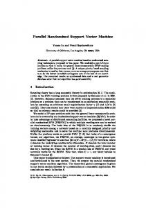
this design philosophy thus they are capable of general purpose computing and referred to as CUDA capable devices. The latest Tesla GPU has the shader processors (cores) fully programmable with large instruction memory, instruction cache and instruction sequencing control logic. Several shader processors share the same instruction cache and instruction sequencing control logic. The Tesla architecture introduced a more generic parallel programming model with a hierarchy of parallel threads, barrier synchronization and atomic operations to dispatch and manage highly parallel computing work. Combined with C/C + + compiler, libraries, runtime software and other useful components, CUDA Software Development Kit is offered to developers who do not possess the programming knowledge of graphics applications. With a minimal learning curve of some extended C/C + + syntax and some basic parallel computing techniques, developers can start migrating existing projects using CUDA with NVIDIA GPUs.
(9)
i:⃗ xi ∈S
Computing the outputs of kernel functions are referred to as kernel computations, which are expensive in terms of time cost due to its nature of intensive computation. These operations drastically slow down the training procedure. 3. General purpose computing using graphics processing unit This section briefly introduces the GPU hardware and the CUDA development platform. 3.1. Graphics processing unit GPUs are microprocessors commonly seen on video cards. The main function of GPU is offloading and accelerating the graphics rendering jobs from the CPU. Before 2006, most GPUs were designed in a way that computing resources were partitioned into vertices and pixel shaders. The only way to accessing GPUs is using OpenGL or DirectX. Smart programmers disguised their general computation problems to graphics problems in order to utilize the hardware capability of GPU. In order to overcome this inflexibility, NVIDIA introduced the GeForce 8800 GTX in 2006, which maps the separated programmable graphics stages to an array of unified processors. Fig. 1 shows the shader pipeline of GeForce 8800 GTX GPU. All later GPU products from NVIDIA follow
3.2. Computing unified device architecture CUDA is a software platform developed by NVIDIA to support their general purpose computing GPUs for easy programming and porting existing applications to GPUs. It primarily uses C/C + + syntax and a few new keywords as an extension, which offers a very low learning curve for an application designer. CUDA memory model and thread organization is introduced in this part. Fig. 2 shows the memory model of the CUDA device. The threads are organized in a hierarchical structure. The top level is a grid which contains blocks of threads. Each grid can contain at most 65,535 blocks in either x- or y-dimension or both in total. Each block can contain at most 1024 (Fermi series) or 512 threads in either x- or y-dimension, or maximally 64 in z-dimension. The total number of threads in all three dimensions must be less than or equal to 1024 or 512 depending on the hardware specification. The organization of threads is shown in Fig. 3. The host (CPU) launches the kernel function on the device (GPU) in the form of grid structure. Once the computation is done, the device becomes available again then the host can launch another kernel function. If multiple devices are available at the same time, every kernel function can be managed through one CPU thread. It is fairly easy to launch a grid structure containing thousands of threads. The optimum number of thread and block configuration varies among different applications. To achieve better performance, there should be at least thousands or tens of thousands of threads with in one
296
Q. Li et al. / J. Parallel Distrib. Comput. 73 (2013) 293–302
Fig. 2. CUDA device memory model. (Courtesy to NVIDIA.)
grid. It would not make much sense to use too few threads to extract maximal performance from hardware. However, too many threads whose number exceeds the number of data would also increase the thread overhead and bring down the efficiency. The multiprocessor creates, manages, schedules, and executes threads in groups of 32 parallel threads called warps. Thus a multiple of 32 could be a good candidate value for the optimal number of threads per block. Threads within the same block have limited shared memory and they are able to communicate with each other by using these shared memory. All threads have their own registers and access to the global memory as well as the constant memory. The size of the global memory can be as large as up to 6 GB (depending on the GPU hardware). Similar to MPI, there is no shared memory between host and device thus the data must be transferred from the host memory to device memory in the first place. The result must also be transferred back for future processing or storage. 4. CUDA implementation of multitask cross validation for SVM This section introduces how to integrate the multitask cross validation in the binary SVM algorithm using CUDA. 4.1. Cross validation The n-fold cross validation is a procedure to locate the best hyperparameters (penalty value C , Gaussian RBF kernel shape value γ and the order of polynomial kernel d) for SVM. For example, a 5-fold cross validation procedure splits the training data set equally into five smaller sets. During each fold of the training phase, every small set is used as the testing data set once and the remaining sets are used for training. The total
number of misclassified samples is accumulated to compute the final accuracy. For example, a Gaussian RBF SVM has two hyperparameters, the penalty value C and the shape parameter γ . If there are 10 different C values and 5 different γ values, the 5-fold cross validation procedure will run 50 times, which are 250 training runs and 250 testing runs. We have mentioned that the kernel computations are expensive in terms of time cost in Section 2. During the training phase, even the simplest linear kernel requires a matrix–vector multiplication for each support vector. Nonlinear kernel computations will cost more due to the complexity of the kernel functions. On the other hand, it is unwise and impossible to compute the complete kernel matrix in advance, because the order of the square kernel matrix is equal to the total number of training samples. There is not enough memory space for storing the complete kernel matrix in general, nor are all training samples used as support vector. Many SVM applications tend to compute the kernel values during the training and store a portion of complete kernel matrix in the system memory for later access. They do cross validation as independent tasks one by one in a sequential manner as shown in the upper part of Fig. 4. In this way, when each training task is completed, its cached kernel values are removed from the memory. This causes duplicated kernel computations across different tasks for different hyperparameters. Fig. 5 shows a binary SVM problem trained with different C . The data set used is an artificial data set which has two overlapped classes with normal distribution. The linear kernel is used in this example and the penalty value C is the only hyperparameter. It is easy to observe from the figure that all four tasks with different C values share certain support vectors. These shared support vectors are shown in Fig. 6. The kernel computations for these shared support vectors are redundant and calculated at least four times in total assuming they are all cached in the memory. The total
Q. Li et al. / J. Parallel Distrib. Comput. 73 (2013) 293–302
297
Fig. 3. CUDA thread organization. (Courtesy to NVIDIA.)
amount of duplicated kernel computations scales with the number of C values used in the cross validation procedure. This is the exact case of running cross validation procedure. However, all these cached kernel values can be shared across different tasks to remove the duplicated kernel computations if they are trained together. Here, we propose a parallel mechanism for cross validation using GPU shown in the lower part of Fig. 4. The n-fold cross validation is done in the following way. All penalty values C ∈ {C1 , . . . , C10 } are grouped together for training. The testing procedure is also parallelized. Therefore, the total number of training runs reduces to 25 and so does the total number of testing runs. Our tests have shown that the time cost for the grouped C training is very close to the time cost for the slowest C trained alone. More results can be found in Section 5. 4.2. The parallel SMO algorithm Cao et al. [3] developed the PSMO algorithm to accelerate binary SVM training by partitioning the input data set and splitting it across multiple computing nodes. Herrero-Lopez et al. [12] further improved it and developed the P2SMO algorithm for multi-class
SVM. In P2SMO, each task is a standalone binary classification problem. Our implementation uses the merits from these two algorithms but extends them for optimizing the cross validation procedure. 4.2.1. The foundation of SMO Define the following index sets at a given α and y: I0 = {i : 0 < αi < C }, I1 = {i : yi = 1, αi = 0}, I2 = {i : yi = −1, αi = C }, I3 = {i : yi = 1, αi = C }, I4 = {i : yi = −1, αi = 0}, Iup = I0 ∪ I1 ∪ I2 , Ilo = I0 ∪ I3 ∪ I4 . The KKT conditions can be rewritten as
∀i ∈ Iup : b ≤ ei , ∀i ∈ Ilo : b ≥ ei ,
298
Q. Li et al. / J. Parallel Distrib. Comput. 73 (2013) 293–302
Fig. 4. 5-fold cross validation steps for Gaussian kernels.
Fig. 5. Linear binary SVM training on the same data set with different C .
Q. Li et al. / J. Parallel Distrib. Comput. 73 (2013) 293–302
Fig. 6. Same support vectors shared among the four tasks in Fig. 5.
where ei =
αj yj K (⃗xj , ⃗xi ) − yi ,
(10)
j:⃗ xj ∈S
thus the KKT conditions will hold if and only if bup = min{ei : i ∈ Iup }, blo = max{ei : i ∈ Ilo }, blo ≤ bup .
(11)
An index pair (i, j) violates the KKT condition if i ∈ Ilo ,
j ∈ Iup
ei > ej ,
and
(12)
thus the objective is eliminating all (i, j) pairs which violate the KKT condition. However, it is usually not possible to achieve the exact optimality conditions. Thus, it is necessary to define the approximate optimality conditions. This is shown in the following equation: blo ≤ bup + 2τ ,
(13)
where τ is a positive tolerance parameter. It is usually set to 0.001 for general applications recommended in [20]. The bias value can be computed by b=
blo + bup 2
.
(14)
In each iteration of the training phase, the α values are updated by s = yup ylo ,
(15)
η = K (⃗xlo , ⃗xlo ) + K (⃗xup , ⃗xup ) − 2K (⃗xlo , ⃗xup ),
(16)
new αup = αup + new lo
α
yup (elo − eup )
η new up
= αlo + s(αup − α
,
).
4.2.2. Multitask cross validation algorithm Data level parallelism is considered within one single binary classification task. The training sample is split into P subsets, which are mapped to P blocks on the GPU. The initialization of αi and p ei are done on the device. After the initialization is completed, p p p p each block computes their local bup , blo , iup , ilo using reduction technique. iup and ilo are the corresponding indexes for bup and blo . Then the global bup , blo , iup , ilo are computed on the CPU. These global values can also be computed on the GPU using single block structure, but it is much more efficient to do this using the CPU because of its smaller scale. Multiple tasks are used for training the data set with several different penalty values simultaneously. Each task is marked with a superscript k and it has its own penalty value C . Each run of the loop is one iteration to minimize the objective function. The optimality condition is set the same as the one used in the sequential algorithm. The difference is that this optimality condition must be met for all tasks to converge. At each iteration of the loop, every task looks at other tasks and checks if other’s current violators are the same as its own ones. These operations are synchronized by the CPU. If the violators are shared in other tasks, the related kernel values are cached in the memory and they can be fetched directly. Otherwise, the CPU will launch the GPU routine to compute those kernel values and the cache will be updated. The fast calculation of kernel values on GPU is the core acceleration part of the SVM algorithm. This is because of the computational complexity of the kernel functions. However, the multitask cross validation training with different hyperparameters eliminates some of these unnecessary kernel computations, which reduces the time cost for the cross validation training significantly. Algorithm 1 Parallel cross validation.
αik = 0, eki ,p = −yki (device) k,p k,p k,p k,p compute bup , blo , iup , ilo (device) k k compute bup , blo , ikup , oklo (host) while bklo > bkup + 2τ do ∀p, q ∈ [1, k] and p, q ∈ Z p q p q p q p q if iup = iup ∥ iup = ilo ∥ ilo = iup ∥ ilo = ilo then fetch kernel values from GPU memory else compute Kik ,ik , Kik ,ik , Kik ,ik (device) lo lo
up up
end if update αik , αik (device) up
k,p
lo
k,p
k,p
up lo
k,p
compute bup , blo , iup , ilo (device) compute bkup , bklo , ikup , iklo (host) end while use αik to test the testing set return number of misclassified testing samples in a vector for this task C = [C1 , . . . , Ck ]
4.3. Cache design (17) (18)
After new α values are computed, the error vector for all training data must be updated by w ene = ei + (αlonew − αlo )ylo K (⃗xlo , ⃗xi ) i new + (αup − αup )yup K (⃗xup , ⃗xi ).
299
(19)
Most kernel values are cached in the GPU device memory, which depends upon the available memory space. In general, the larger the device memory is, the better the performance should be.
There are two layers in the cache shown in Fig. 7. They are the abstract layer and the physical layer. The abstract layer is used as a programming interface to maintain the Least Recently Used (LRU) list which is on the CPU side. The physical layer is the GPU device memory layout. A 2D array referred to as cache array on the GPU device is used as the storage of kernel matrix. Each row stores a kernel vector containing kernel values from one support vector to all data points. Thus the number of columns is fixed to the number of all data points and the number of rows is the size of the cache, which depends upon the available memory on the GPU device. The abstract layer contains a vector of nodes and a LRU list. Each nodes includes information about status, location and lrulistpos.
300
Q. Li et al. / J. Parallel Distrib. Comput. 73 (2013) 293–302
Fig. 7. The cache structure design.
Each node represents a data point, status indicates whether the node is in the LRU list; location stores the row number of cache array on the GPU device; lrulistpos stores the position of the node in the LRU list. The LRU list has the same size as the cache. There are two different scenarios of doing operations on the cache: 1. The new support vector is in the cache. If lrulistpos points at the head of LRU list, do nothing and return its location. If not, remove it from the LRU list and append it back to the head of LRU list. Update the its lrulistpos and return its location. The GPU fetches the kernel vector from the location directly. 2. The new support vector is not in the cache. (a) If the cache is not full, append the new support vector at the head of the LRU list and update its lrulistpos. Increase the size of the LRU list by 1 and set the new support vector’s location to the value of LRU list’s size after the increment. Set its status to IN, return its location and ask for kernel computation. The GPU computes the kernel vector and stores it in the location on the GPU device memory. This operation overwrites a blank space. (b) If the cache is full, retrieve the support vector from the end of the LRU list and assign its location value to the new support vector’s location. Set the expired support vector’s status to OUT. Remove the expired support vector from the LRU list and append the new support vector at the head of the LRU list. Update the lrulistpos of the new support vector and set its status to IN. Return its location and ask for the kernel computations. The GPU computes the kernel vector and stores it in the location on the GPU device memory. This operation overwrites the memory space used by the expired support vector. By carrying out the above operations, the most recently used support vector will always appear at the head of the LRU list. Whenever the cache is full, the erased point is always the least recently used support vector. This cache design minimizes the unnecessary kernel computations within one single binary task as well as multitask cross validation. If the cache size is large enough, kernel vectors of all support vectors appeared during training are only computed once.
Table 2 The experimental data sets and their hyperparameters for the Gaussian RBF kernel. Data set
# of training samples
# of testing samples
# of features
C
γ
Heart Sonar Breast-cancer Adult Web
270 208 683 32,561 49,749
N/A N/A N/A 16,281 14,951
13 60 10 123 300
0.5 4 0.25 1 64
0.0625 0.125 0.125 0.0625 8
5. Experimental results This section presents the performance results obtained by the proposed algorithm. The routines are developed using CUDA in C/C + +. The following measurements are carried out by our latest workstation computer equipped with two Intel Xeon X5680 3.3 GHz six-core CPUs, 96 GB ECC DDR3 1333 MHz main memory, six Tesla C2050 with 3 GB GDDR5 memory each and two Tesla C2070 with 6 GB GDDR5 memory each. The storage device is a 128 GB SSD with Fedora Core Linux 14 × 64 installed. The CUDA driver and runtime version are both 3.2. Only one Telsa C2070 card is used in all benchmark tests. 5.1. Data sets All data sets used in the experiments are downloaded from the official LIBSVM website with pre-scaled values. The characteristics of the data sets and the hyperparameters used for the Gaussian RBF kernel are listed in Table 2. They are all binary class data sets. Sonar, breast-cancer, adult data sets are originally from UCI [10] and heart data set is from Statlog [21]. Web is web pages text categorization used in [20]. The hyperparameter C is the penalty value and γ is the shape value of RBF kernel. The best hyperparameters for each data set are listed for the sake of accuracy verification. And they are discovered by using 5-fold cross validation on C ∈ {2i , i ∈ [−10, 10] and i ∈ Z}, γ ∈ {2i , i ∈ [−5, 5] and i ∈ Z}.
Q. Li et al. / J. Parallel Distrib. Comput. 73 (2013) 293–302
301
Fig. 8. Independent task comparison between GPUSVM and LIBSVM. Table 3 The accuracy comparison between GPUSVM and LIBSVM on the experimental data sets. Data set
SVM
Training accuracy (%)
Predicting accuracy (%)
# of support vectors
N/A
146 146
Heart
LIBSVM GPUSVM
85.1852 85.1852
Sonar
LIBSVM GPUSVM
100 100
N/A
150 150
Breast-cancer
LIBSVM GPUSVM
97.2182 97.2182
N/A
91 91
Adult
LIBSVM GPUSVM
85.7928 85.7928
85.0132 85.0193
11,647 11,587
Web
LIBSVM GPUSVM
99.4553 99.4553
99.4515 99.4515
35,231 35,220
5.2. Accuracy verification The proposed method is trained and tested by using one set of C and γ values to verify the accuracy performance on the given data sets. Both the accuracies obtained for training set and testing set are given compared to the results obtained using the LIBSVM tool shown in Table 3. There is only one task running in this scenario. We denote the GPU method as GPUSVM-S. It can be readily seen that the accuracy performance of our proposed method is as good as LIBSVM. For small data set, GPUSVM-S has the exact same number of support vectors as LIBSVM does. They also have the same accuracy. However, they get a slightly different number of support vectors for large data sets and the accuracy performances also have very small differences. One possible explanation for this tiny difference can be that the precisions offered by the basic math functions (e.g., exponential function) from CPU and GPU are different. The implementations of LIBSVM second order heuristics and shrinking techniques may also cause the differences in the final results. Nevertheless, both tools present excellent classification accuracy. 5.3. Speed performance analysis Only adult and web data sets are measured for speed performance. The other data sets are considerably small and their training time costs are trivial. Table 4 shows the comparison of the training time cost between GPUSVM-S, GPUSVM-P and
Table 4 The speed comparison between GPUSVM-S, GPUSVM-P and LIBSVM. Data set
SVM
Training time (s)
Speedup
Adult
LIBSVM GPUSVM-S GPUSVM-P
1601.37 309.91 155.42
1x 5.2x 10.3x
Web
LIBSVM GPUSVM-S GPUSVM-P
12198.3 564.16 123.36
1x 21.6x 98.9x
LIBSVM. GPUSVM-S is single task training as mentioned before and it trains a pair of C and γ one by one on GPU. GPUSVMP uses the proposed method to train all C and one γ together. LIBSVM trains a pair of C and γ one by one which is the same as what GPUSVM-S does. For adult data set, the γ = 0.0625 and C ∈ {0.125, 0.25, 0.5, 1, 2, 4, 8, 16, 32, 64}. For web data set, the γ = 8 and C ∈ {0.125, 0.25, 0.5, 1, 2, 4, 8, 16, 32, 64}. The performance of LIBSVM is set as the baseline. GPUSVM-P gets 10 times faster on adult data set and almost 100 times faster on web data set for SVM training. In order to analyze the performance result in more detail, Fig. 8 shows the independent task comparison between LIBSVM and GPUSVM-S. Both of them are measured with 10 pairs of different combinations of C and γ values in 10 tasks. GPUSVM-S shows good speed improvement on every independent task. The total number of support vectors of GPUSVM-S and LIBSVM is very close in each task, which guarantees the accuracy performance. The support vectors and their related α obtained by GPUSVM-P are identical to GPUSVM-S. The total number of kernel computations are shown in Fig. 9. The duplicated kernel computations in GPUSVM-S lead to a longer training time compared to GPUSVM-P. 6. Conclusions In summary, the proposed GPUSVM shows excellent speed improvement compared to the state of the art LIBSVM tool. It has as good performance as LIBSVM in terms of classification accuracy. The speed improvement is further increased by involving multitask training for different hyperparameters in the cross validation procedure. The standard cross validation procedure suffers from the slow training because of the redundant computations of kernel values across multiple tasks in the traditional setting. The proposed GPUSVM resolves this issue by parallel executing several training
302
Q. Li et al. / J. Parallel Distrib. Comput. 73 (2013) 293–302 [17] S.S. Keerthi, S.K. Shevade, C. Bhattacharyya, K.R.K. Murthy, Improvements to platt’s smo algorithm for svm classifier design, Neural Computation 13 (3) (2001) 637–649. [18] NVIDIA, CUDA CUBLAS Library, June 2007. [19] E. Osuna, R. Freund, F. Girosi, An improved training algorithm for support vector machines, in: Neural Networks for Signal Processing [1997] VII. Proceedings of the 1997 IEEE Workshop, 1997, pp. 276–285. [20] J.C. Platt, Fast Training of Support Vector Machines Using Sequential Minimal Optimization, MIT Press, Cambridge, MA, USA, 1999, pp. 185–208. [21] LIACC, Statlog datasets, 2010. URL http://www.liacc.up.pt/. [22] M. Stone, Cross-validatory choice and assessment of statistical predictions, Journal of the Royal Statistical Society. Series B (Methodological) 36 (2) (1974) 111–147. [23] V.N. Vapnik, The Nature of Statistical Learning Theory, Springer, 2000. [24] G. Zanghirati, L. Zanni, A parallel solver for large quadratic programs in training support vector machines, Parallel Computing 29 (2003) 535–551.
Fig. 9. Total number of kernel computations for GPUSVM-S and GPUSVM-P.
tasks simultaneously and all tasks can share the same cache memory for storing kernel values. In this manner, most duplicated kernel computations across different tasks are eliminated. The speed performance is expected to be better on the GPU device that has a larger physical memory. The next extension of this work will be using multiple GPU devices to solve even larger SVM training problem in parallel fashion. References [1] A. Athanasopoulos, A. Dimou, V. Mezaris, I. Kompatsiaris, Gpu acceleration for support vector machines, in: Image Analysis for Multimedia Interactive Services, WIAMIS 2011, 12th International Workshop on, 2010. [2] Y. Bengio, Y. Grandvalet, No unbiased estimator of the variance of k-fold crossvalidation, Journal of Machine Learning Research 5 (2004) 1089–1105. [3] L.J. Cao, S.S. Keerthi, C.-J. Ong, J.Q. Zhang, U. Periyathamby, X.J. Fu, H.P. Lee, Parallel sequential minimal optimization for the training of support vector machines, Neural Networks, IEEE Transactions on 17 (4) (2006) 1039–1049. [4] B. Catanzaro, N. Sundaram, K. Keutzer, Fast support vector machine training and classification on graphics processors, in: Proceedings of the 25th International Conference on Machine Learning, ICML ’08, ACM, New York, NY, USA, 2008, pp. 104–111. [5] C.-C. Chang, C.-J. Lin, LIBSVM: a library for support vector machines, 2001. Software available at http://www.csie.ntu.edu.tw/~cjlin/libsvm. [6] R. Collobert, S. Bengio, Y. Bengio, A parallel mixture of svms for very large scale problems, Neural Computation 14 (5) (2002) 1105–1114. [7] C. Cortes, V. Vapnik, Support-vector networks, Machine Learning 20 (1995) 273–297. [8] J.-X. Dong, A. Krzyżak, C.-Y. Suen, A fast parallel optimization for training support vector machine, in: Machine Learning and Data Mining in Pattern Recognition, in: Lecture Notes in Computer Science, vol. 2734, Springer, Berlin, Heidelberg, 2003, pp. 96–105. [9] R.-E. Fan, P.-H. Chen, C.-J. Lin, Working set selection using second order information for training support vector machines, Journal of Machine Learning Research 6 (2005) 1889–1918. [10] A. Frank, A. Asuncion, UCI machine learning repository, 2010. URL http://archive.ics.uci.edu/ml. [11] H.P. Graf, E. Cosatto, L. Bottou, I. Durdanovic, V. Vapnik, Parallel support vector machines: the cascade svm, in: In Advances in Neural Information Processing Systems, MIT Press, 2005, pp. 521–528. [12] S. Herrero-Lopez, J.R. Williams, A. Sanchez, Parallel multiclass classification using svms on gpus, in: Proceedings of the 3rd Workshop on General-Purpose Computation on Graphics Processing Units, GPGPU ’10, ACM, New York, NY, USA, 2010, pp. 2–11. [13] W.D. Hillis, G.L. Steele Jr., Data parallel algorithms, Communications of the ACM 29 (1986) 1170–1183. [14] T.-M. Huang, V. Kecman, I. Kopriva, Kernel Based Algorithms for Mining Huge Data Sets: Supervised, Semi-supervised, and Unsupervised Learning, Springer, 2006. [15] G.-B. Huang, K.Z. Mao, C.-K. Siew, D.-S. Huang, Fast modular network implementation for support vector machines, Neural Networks, IEEE Transactions on 16 (6) (2005) 1651–1663. [16] T. Joachims, Making Large-Scale Ssupport Vector Machine Learning Practical, MIT Press, Cambridge, MA, USA, 1999, pp. 169–184.
Qi Li received his B.S. Degree in Electronic Engineering from Beijing University of Posts and Telecommunications, Beijing, China, in 2007 and M.S. Degree in Computer Science from Virginia Commonwealth University, Richmond, United States, in 2008. He is now a Ph.D. candidate in Computer Science at Virginia Commonwealth University. His research interests include data mining and parallel computing using GPU.
Raied Salman received the B.S. Degree (with high distinction) in Electrical Engineering and M.S. Degree in Computer Control from the University of Technology, Baghdad, Iraq in 1976 and 1978, respectively. He also received the Ph.D. in Electrical Engineering from Brunel University, England, UK in 1989. He is currently a Ph.D. candidate in the Department of Computer Science at Virginia Commonwealth University, Richmond, VA. His research interests include machine learning and data mining for large data sets.
Erik Test is a Ph.D. student at Virginia Commonwealth University (VCU), Richmond, United States studying Computer Science and will complete his Master’s Degree in May, 2011. He received his Bachelor’s Degree in Computer Science in 2007 from VCU. He also gained previous work experience at Acision, BAE Systems, and SENTEL. His research interests are high performance computing (HPC), GPU computing, and machine learning as well as machine learning in an HPC framework.
Robert Strack received his M.S. Eng. Degree in Computer Science from AGH University of Science and Technology, Cracow, Poland in 2007. He is now working towards his Ph.D. Degree in Computer Science at Virginia Commonwealth University, Richmond, US. His research is oriented towards machine learning and data mining algorithms and his field of interest includes Support Vector Machine classification and parallel computing.
Vojislav Kecman is with VCU, Dept. of CS, Richmond, VA, USA, working in the fields of machine learning by both Support Vector Machines (SVMs) and neural networks, as well as by local approaches such as Adaptive Local Hyperplane (ALH) and Local SVMs, in different regression (function approximation) and pattern recognition (classification, decision making) tasks. He was a Fulbright Professor at MIT, Cambridge, MA, a Konrad Zuse Professor at FH Heilbronn, DFG Scientist at TU Darmstadt, a Research Fellow at Drexel University, Philadelphia, PA, and at Stuttgart University. Dr. Kecman authored several books on ML (see www.supportvector.ws and www.learning-from-data.com).