information has received increasing attention in the recent years. A number of ... vantage of neural networks, on the other hand, is the inherent learning capability, ... The paper finishes with some conclusions and pointers to future work. ... A Neural Implementation of Multi-Adjoint Programs Via sf-homogenization 201.
Mathware & Soft Computing 12 (2005) 199-216
A Neural Implementation of Multi-Adjoint Logic Programs Via sf-homogenization J. Medina, E. M´erida-Casermeiro, M. Ojeda-Aciego Dept. Matem´atica Aplicada. Universidad de M´alaga∗ {jmedina,merida,aciego}@ctima.uma.es
Abstract A generalization of the homogenization process needed for the neural implementation of multi-adjoint logic programming (a unifying theory to deal with uncertainty, imprecise data or incomplete information) is presented here. The idea is to allow to represent a more general family of adjoint pairs, but maintaining the advantage of the existing implementation recently introduced in [6]. The soundness of the transformation is proved and its complexity is analysed. In addition, the corresponding generalization of the neural-like implementation of the fixed point semantics of multi-adjoint is presented.
1
Introduction
The study of reasoning methods under uncertainty, imprecise data or incomplete information has received increasing attention in the recent years. A number of different approaches have been proposed with the aim of better explaining observed facts, specifying statements, reasoning and/or executing programs under some type of uncertainty whatever it might be. One important and powerful mathematical tool that has been used for this purpose at theoretical level is fuzzy logic. From the applicative side, neural networks have a massively parallel architecture-based dynamics which are inspired by the structure of human brain, adaptation capabilities, and fault tolerance. The recent paradigm of soft computing promotes the use and integration of different approaches for the problem solving. The main advantages of fuzzy logic systems are the capability to express nonlinear input/output relationships by a set of qualitative if-then rules, and to handle both numerical data and linguistic knowledge, especially the latter, which is extremely difficult to quantify by means of traditional mathematics. The main advantage of neural networks, on the other hand, is the inherent learning capability, which enables the networks to adaptively improve their performance. ∗ Partially
supported by TIC2003-09001-C02-01.
199
200
J. Medina, E. M´erida-Casermeiro & M. Ojeda-Aciego
Recently, a new approach presented in [6] introduced a hybrid framework to handling uncertainty, expressed in the language of multi-adjoint logic but implemented by using ideas from the world of neural networks. The handling of uncertainty inside their logic model is based on the use of a generalised set of truth-values as a generalization of [11]. On the other hand, multi-adjoint logic programming [8] generalizes residuated logic programming [1] in that several different implications are allowed in the same program, as a means to facilitate the task of specification. Considering several implications in the same program is interesting because it provides a more flexible framework for the specification of problems, for instance, in situations in which connectives are built from the users preferences. In these contexts, it is likely that knowledge is described by a many-valued logic program where connectives have many-valued truth functions and, perhaps, aggregation operators (such as arithmetic mean or weighted sum) where different implications could be needed for different purposes, and different aggregators are defined for different users, depending on their preferences. The neural-like implementation of multi-adjoint logic programming in [6] had the restriction that the only connectives involved in the program were the usual product, G¨ odel and Lukasiewicz together with weighted sums. A key point of the implementation was a preprocessing of the initial program to transform it into a homogeneous program. As the theoretical development of the multi-adjoint framework does not rely on particular properties of the product, G¨ odel and Lukasiewicz adjoint pairs, it seems convenient to allow for a generalization of the implementation to admit, at least, a family of continuous t-norms (recall that any continuous t-norm can be interpreted as the ordinal sum of product and Lukasiewicz t-norms). The authors presented in [7] a different neural approach allowing for ordinal sums in the initial program, which uses the same homogenization process introduced in [6]. The purpose of this paper is to present a “finer” homogenization process for multi-adjoint logic programs such that conjunctors which are built as ordinal sums of product, G¨ odel and Lukasiewicz t-norms are decomposed into its components so that, as a result, the original neural approach is still applicable. The structure of the paper is as follows: In Section 2, the syntax and semantics of multi-adjoint logic programs are introduced, together with the homogenization procedure; in Section 3, the translation from multi-adjoint programs into homogeneous programs is extended in order to cope with conjunctors defined as ordinal sums, the preservation of the semantics is proved under this extended transformation, and the complexity of the translation is studied. Section 4 introduces the modification of the neural net of [6] in order to include the modification of the homogenization process and the comparison with the sequence of iterations of the TP operator is presented; then, some comments about related approaches are given in Section 5. The paper finishes with some conclusions and pointers to future work.
2
Preliminary definitions
To make this paper as self-contained as possible, the necessary definitions about multi-adjoint structures are included in this section. For motivating comments, the
A Neural Implementation of Multi-Adjoint Programs Via sf-homogenization 201
interested reader is referred to [8]. Multi-adjoint logic programming is a general theory of logic programming which allows the simultaneous use of different implications in the rules and rather general connectives in the bodies. The first interesting feature of multi-adjoint logic programs is that a number of different implications are allowed in the bodies of the rules. The basic definition is the generalization of residuated lattice given below: Definition 1 A multi-adjoint lattice L is a tuple (L, �, ←1 , &1 , . . . , ←n , &n ) satisfying the following items: 1. hL, �i is a bounded lattice, i.e. it has bottom and top elements; 2. ⊤ &i ϑ = ϑ &i ⊤ = ϑ for all ϑ ∈ L for i = 1, . . . , n; 3. (&i , ←i ) is an adjoint pair in hL, �i for i = 1, . . . , n; i.e. (a) Operation &i is increasing in both arguments, (b) Operation ←i is increasing in the first argument and decreasing in the second argument, (c) For any x, y, z ∈ P , we have that x � (y ←i z) holds if and only if (x &i z) � y holds. In the rest of the paper we restrict to the unit interval, although the general framework of multi-adjoint logic programming is applicable to a general lattice.
2.1
Syntax of multi-adjoint logic programs
A multi-adjoint program is a set of weighted rules hF, ϑi satisfying the following conditions: 1. F is a formula of the form A ←i B where A is a propositional symbol called the head of the rule, and B is a well-formed formula, which is called the body, built from propositional symbols B1 , . . . , Bn (n ≥ 0) by the use of monotone operators. 2. The weight ϑ is an element (a truth-value) of [0, 1]. Facts are rules with body1 1 and a query (or goal ) is a propositional symbol intended as a question ?A prompting the system.
2.2
Semantics of multi-adjoint logic programs
Once presented the syntax of multi-adjoint programs, the semantics is given below. Definition 2 An interpretation is a mapping I from the set of propositional symbols Π to the lattice h[0, 1], ≤i. 1 It
is also customary to use write ⊤ instead of 1, and even not to write any body.
202
J. Medina, E. M´erida-Casermeiro & M. Ojeda-Aciego
Note that each of these interpretations can be uniquely extended to the whole set ˆ The set of all the interpretations of formulas, and this extension is denoted as I. is denoted IL . The ordering ≤ of the truth-values L can be easily extended to IL , which also inherits the structure of complete lattice and is denoted ⊑. The minimum element of the lattice IL , which assigns 0 to any propositional symbol, will be denoted △. Definition 3 1. An interpretation I ∈ IL satisfies hA ←i B, ϑi if and only if ϑ ≤ Iˆ (A ←i B). 2. An interpretation I ∈ IL is a model of a multi-adjoint logic program P iff all weighted rules in P are satisfied by I. The operational approach to multi-adjoint logic programs used in this paper will be based on the fixpoint semantics provided by the immediate consequences operator, given in the classical case by van Emden and Kowalski [10], which can be generalised to the framework of multi-adjoint logic programs by means of the adjoint property, as shown below: Definition 4 Let P be a multi-adjoint program; the immediate consequences operator, TP : IL → IL , maps interpretations to interpretations, and for I ∈ IL and A ∈ Π is given by n o ˆ TP (I)(A) = sup ϑ &i I(B) | hA ←i B, ϑi ∈ P
As usual, it is possible to characterise the semantics of a multi-adjoint logic program by the post-fixpoints of TP ; that is, an interpretation I is a model of a multi-adjoint logic program P iff TP (I) ⊑ I. The TP operator is proved to be monotonic and continuous under very general hypotheses. Once one knows that TP can be continuous under very general hypotheses [8], then the least model can be reached in at most countably many iterations beginning with the least interpretation, that is, the least model is TP ↑ ω(△).
2.3
Obtaining a homogeneous program
Regarding the implementation as a neural network of [6], the introduction of the so-called homogeneous rules, provided a simpler and standard representation for any multi-adjoint program. Definition 5 A weighted formula is said to be homogeneous if it has one of the following forms: • hA ←i &i (B1 , . . . , Bn ), ϑi • hA ←i @(B1 , . . . , Bn ), 1i • hA ←i B1 , ϑi
A Neural Implementation of Multi-Adjoint Programs Via sf-homogenization 203
where A, B1 , . . . , Bn are propositional symbols. In the rest of this section we briefly recall the procedure for translating a multiadjoint logic program into one containing only homogeneous rules. The procedure handles separately rules and facts, the latter are not related to the purpose of this paper, therefore we will only recall the procedure presented for homogenizing rules. Two types of transformations are considered: The first one handles the main connective of the body of the rule, whereas the second one handles the subcomponents of the body. T 1. A weighted rule hA ←i &j (B1 , . . . , Bn ), ϑi is substituted by the following pair of formulas: hA ←i A1 , ϑi hA1 ←j &j (B1 , . . . , Bn ), 1i where A1 is a fresh propositional symbol, and h←j , &j i is an adjoint pair. For the case hA ←i @(B1 , . . . , Bn ), ϑi in which the main connective of the body of the rule happens to be an aggregator, the transformation is similar: hA ←i A1 , ϑi hA1 ← @(B1 , . . . , Bn ), 1i where A1 is a fresh propositional symbol, and ← is a designated implication. T 2. A weighted rule hA ←i Θ(B1 , . . . , Bn ), ϑi, where Θ is either &i or an aggregator, and a component Bk is assumed to be either of the form &j (C1 , . . . , Cl ) or @(C1 , . . . , Cl ), is substituted by the following pair of formulas in either case: hA ←i Θ(B1 , . . . , Bk−1 , A1 , Bk+1 , . . . , Bn ), ϑi hA1 ←j &j (C1 , . . . , Cl ), 1i or hA ←i Θ(B1 , . . . , Bk−1 , A1 , Bk+1 , . . . , Bn ), ϑi hA1 ← @(C1 , . . . , Cl ), 1i where A1 is a fresh propositional symbol. The procedure to transform the rules of a program so that all the resulting rules are homogeneous, is presented in Fig. 1. It is based in the two previous transformations, and in its description by abuse of notation the terms T1-rule (resp. T2-rule) are used to mean an adequate input rule for transformation T1 (resp. T2).
204
J. Medina, E. M´erida-Casermeiro & M. Ojeda-Aciego Program Homogenization begin repeat for each T1-rule do Apply transformation T1 end-for for each T2-rule do Apply transformation T2 end-for until neither T1-rules nor T2-rules exist end Figure 1: Pseudo-code for translating into a homogeneous program.
3
Considering compound conjunctors
As stated in the introduction, a neural net implementation of the immediate consequences operator of an homogeneous program was introduced in [6] for the case of the multi-adjoint lattice ([0, 1], ≤, &P , ←P , &G , ←G , &L , ←L ). As the theoretical development of the multi-adjoint framework does not rely on particular properties of these three adjoint pairs, it seems convenient to allow for a generalization of the implementation to, at least, a family of continuous t-norms, for any continuous t-norm can be interpreted as the ordinal sum of product and Lukasiewicz t-norms. In order to maintain the most of the proposed implementation, it makes sense to consider an extra process in the homogenization process in order to further translate a program with new types of t-norms into one on which the original neural approach is still applicable. Recall the definition of ordinal sum of a family of t-norms: Definition 6 Let (&i )i∈Λ be a family of t-norms and a family of non-empty pairwise disjoint subintervals [ai , bi ] of [0, 1]. The ordinal sum of the summands (ai , bi , &i ), i ∈ Λ is the t-norm & defined as ( i , y−ai ) x, y ∈ [ai , bi ] ai + (bi − ai ) &i ( bx−a i −ai bi −ai &(x, y) = min(x, y) otherwise In order to simplify the notation of ordinal sum, let us introduce suitable functions for change of scale, to be able to switch between the intervals [0, 1] and [ai , bi ]. Given the unit interval [0, 1] and a subset [ai , bi ] ⊆ [0, 1], the function fi : [ai , bi ] → [0, 1], with fi (x) =
x − ai b i − ai
is bijective, and its inverse is fi−1 : [0, 1] → [ai , bi ], with fi−1 (x) = ai + (bi − ai )x
A Neural Implementation of Multi-Adjoint Programs Via sf-homogenization 205 Now, given a t-norm &i consider the following (adapted) t-norm2 : � −1 fi (fi (x) &i fi (y)) if x, y ∈ [ai , bi ] ∗ x &i y = min{x, y} otherwise
(1)
for all x, y ∈ [0, 1]. With the notations above it is obvious that the ordinal sum of the summands (ai , bi , &i ), i ∈ Λ can be written as x & y = min{x &∗i y | i ∈ Λ}
(2)
With this expression for the ordinal sum, we can introduce a third type of transformation, to be applied to those rules of a homogeneous program with a finite ordinal sum in the body. i.e. Λ = {1, . . . , n}. T 3. The homogeneous rule3 hA ←s B1 &s B2 , ϑi, where & is expressed as in (2) is substituted by the following n + 1 formulas: hA1 ←∗s B1 &∗1 B2 , ϑi .. . ∗ ∗ hAn ←n B1 &n B2 , ϑi hA ←G &G (A1 , . . . , An ), ϑi where A1 , . . . , An are fresh propositional symbols, and ←∗i are the adjoint implications of &∗i . After applying this transformation to a homogeneous program, we obtain another homogeneous program in whose bodies no t-norm appears as an ordinal sum. This kind of homogenous program is called sum-free homogeneous program (in short sf-homogeneous program). Example 1 Consider the elements a1 = 0.1, b1 ordinal sum &s defined as −1 f1 (f1 (x) &P f1 (y)) x &s y f −1 (f2 (x) &L f2 (y)) 2 min{x, y}
= 0.5, a2 = 0.7, b2 = 0.9 and the if x, y ∈ [a1 , b1 ] if x, y ∈ [a2 , b2 ] otherwise
Then if we have the homogeneous rule hA ←s B1 &s B2 , 1i, applying T3, this is transformed in4 hA1 ←∗P B1 &∗P B2 , 1i sf-homogeneous hAn ←∗L B1 &∗L B2 , 1i sf-homogeneous hA ←G &G (A1 , . . . , An ), 1i sf-homogeneous 2 For
example, if we have that [ai , bi ] = [0, 1] then x &∗P y = x &P y. simplify the presentation, let us assume that the body has just two arguments. 4 Note that it is not necessary to specify the type of the implications in the rules because the weights are 1. Usually, we will omit the subscript in these cases. 3 To
206
J. Medina, E. M´erida-Casermeiro & M. Ojeda-Aciego
The procedure to transform the rules of a program so that all the resulting rules are sf-homogeneous, is presented in Fig. 2. In its description by abuse of notation we use the terms T1-rule (resp. T2-rule, T3-rule) to mean an adequate input rule for transformation T1 (resp. T2, T3). Program sf-Homogenization begin repeat for each T1-rule do Apply transformation T1 end-for for each T2-rule do Apply transformation T2 end-for for each T3-rule do Apply transformation T3 end-for until neither T1- nor T2- nor T3-rules exist end Figure 2: Pseudo-code for translating into a sf-homogeneous program.
3.1
Preservation of the semantics
It is necessary to check that the semantics of the initial program has not been changed by the transformation. The following results will show that every model of the sf-homogenized program P∗ is also a model of the original program P and, in addition, the minimal model of P∗ is also the minimal model of P. Theorem 1 Let P be a homogeneous program, then every model of the program P∗ , obtained after to apply the sf-homogenization process to P, is also a model of P when restricted to the variables occurring in P. Proof: It will be sufficient to show that the transformation T3 satisfies that every model of its output is also a model of its input, as the proof for T1 and T2 was given in [6]. Assume that I is a model of the rules hA1 ← B1 &∗1 B2 , 1i,
...,
hAn ← B1 &∗n B2 , 1i
hA ←G &G (A1 , . . . , An ), 1i therefore we have ˆ 1 &∗ B2 ) ≤ I(Ai ) and I( ˆ &G (A1 , . . . , An )) ≤ I(A) I(B i
A Neural Implementation of Multi-Adjoint Programs Via sf-homogenization 207
for all i ∈ {1, . . . , n}. Now, by monotonicity, we have ˆ 1 &∗ B2 ), . . . , I(B ˆ 1 &∗ B2 )) ≤ I(A) &G (I(B 1 n Recall that we want to prove that I satisfies the rule hA ←i B1 & B2 , 1i, that is, ˆ 1 & B2 ) ≤ I(A), where & is an ordinal sum of &∗ , i ∈ {1, . . . , n}. But this is I(B i true by Equation (2) above, since we have I(B1 ) & I(B2 ) = mini∈{1,...,n} {I(B1 ) &∗i I(B2 )} ˆ 1 &∗ B2 ), . . . , I(B ˆ 1 &∗ B2 )) = &G (I(B 1 n ≤ I(A) qed Theorem 2 Given a program P, the minimal model of the program P∗ obtained after applying sf-homogenization, is also a model of P when restricted to variables in P. The idea underlying the proof is to consider any model I of P, then extend it to P∗ in such a way that it is also a model of P∗ , finally use minimality on P∗ . The key point is to notice that, for every “fresh” propositional variable Ai introduced by the process, there is only one rule headed with Ai in the resulting program. This feature allows the extension of any model I to these new symbols in purely recursive terms. Proof: Let M ∗ be the minimal model of P∗ , and let M denote its restriction to P. By the Theorem 1 we have that M is also a model of P, so we have only to prove that it is minimal. Once again, only the behaviour of transformation T3 has to be taken into account. Given a model I of P, consider a rule hAi ← B1 &∗i B2 , 1i, where Ai is a propositional variable in P∗ but not in P. We argued above that there can be only one such rule headed with Ai , therefore the following extension of I makes sense: ˆ 1 &∗i B2 ) I ∗ (Ai ) = I(B Obviously, by definition this extension I ∗ is also a model of P∗ , therefore the minimal model M ∗ of P∗ satisfies M ∗ ⊑ I ∗ . Now, by restricting the domain back to the variables in P we obtain M ⊑ I. Therefore, M is the minimal model of P. qed
3.2
Complexity issues
In [6] it was shown that the complexity of the algorithm for transforming a multiadjoint program into a homogeneous one is linear on the size of the program. Specifically, the following theorem was stated and proved
208
J. Medina, E. M´erida-Casermeiro & M. Ojeda-Aciego
Theorem 3 Let hA ←i Θ(B1 , . . . , Bl ), ϑi be a rule with n connectives in the body (n ≥ 1), then: • The number of homogeneous rules obtained after applying the procedure is n, if either Θ = &i or Θ = @ with ϑ = 1; and n + 1 otherwise. • The number of transformations applied by the procedure is n − 1 if either Θ = &i or Θ = @ with ϑ = 1; and n otherwise. Back to the sf-homogenization process, it can also be shown to be linear on the size of the program. The following theorem shows a precise calculation of the complexity of the homogenization procedure. Theorem 4 Let hA ←i Θ(B1 , . . . , Bl ), ϑi be a rule with n connectives in the body (n ≥ 1), out of which exactly m are constructed as ordinal sums of ki basic connectives for each i ∈ {1, . . . , m} then: • The number of homogeneous rules obtained after applying the procedure is Pm bounded by n + m + k , if either Θ = &i or Θ = @ with ϑ = 1; and i i=1 Pm n + m + i=1 ki + 1 otherwise.
• The number of transformations Ti applied by the procedure is n + 2m − 1 if either Θ = &i or Θ = @ with ϑ = 1; and n + 2m otherwise.
Proof: Concatenate the thesis of Theorem 3 with the fact that an application of T3 generates exactly k + 1 rules, provided that the ordinal sum was built out of k intervals, because in each homogeneous rule there is only one operator in the body. qed
4
The neural implementation to use ordinal sums
A neural-based implementation of multi-adjoint logic program has already been presented, which is able to calculate the minimal model of a multi-adjoint logic program built solely from product, G¨ odel and Lukasiewicz adjoint pairs and weighted sums. In this section, we introduce an extension which is able to work on programs whose conjunctors are built as finite ordinal sums.
4.1
The structure of the neural net
A neural net is built from a sf-homogeneous program where each process unit is associated either to a propositional symbol of the initial program or to an sfhomogeneous rule. The state of the i-th neuron in the instant t is expressed by its output function, denoted Si (t). The state of the network can be expressed by ~ means of a state vector S(t), whose components are the output of the neurons ~ is 0 for all the components except those forming the network; the initial state of S representing a propositional variable, say A, in which case its value is defined as: ( ϑA if hA ← 1, ϑA i ∈ P, SA (0) = 0 otherwise.
A Neural Implementation of Multi-Adjoint Programs Via sf-homogenization 209
where SA (0) denotes the component associated to a propositional symbol A. The connection between neurons is denoted by a matrix of weights W , in which wkj indicates the existence or absence of connection between unit k and unit j; if the neuron represents a weighted sum, then the matrix of weights also represents the weights associated to any of the inputs. The weights of the connections related to neuron i (that is, the i-th row of the matrix W ) are represented by an n-upla Wi• , and are allocated in an internal vector register of the neuron, which can be seen as a distributed information system. The initial truth-value of the propositional symbol or sf-homogeneous rule vi is loaded in the internal register, together with a signal mi to distinguish whether the neuron is associated either to a fact or to a rule; in the latter case, information about the type of operator is also included. Moreover, it is necessary introduce the (sub-)intervals on which the new connective will be operating, i.e. to set the values of the extremes of interval ai and bi . Therefore, there are four vectors: the first storing the truth-values ~v of atoms and sf-homogeneous rules, the second m ~ storing the type of the neurons in the net and the last two representing the (sub-)intervals of the components of the ordinal sums. A signal mi indicates the functioning mode of the neuron. If mi = 1, then the neuron is assumed to be associated to a propositional symbol, and its next state is the maximum value among all the operators involved in its input, its previous state, and the initial truth-value vi . More precisely: � � Si (t + 1) = max vi , max{Sk (t) | wik > 0} k
Note that for this case, the values introduced as extremes of interval are, naturally, ai = 0 and bi = 1. When a neuron is associated to the product, G¨ odel, or Lukasiewicz implication, respectively, then the signal mi is set to 2, 3, and 4, respectively. Its input is formed by the external value vi of the rule, the outputs of the neurons associated to the body of the implication and the extremes ai , bi of the interval of each connective. The output of the neuron mimics the behaviour of the implication in terms of the adjoint property when a rule of type mi has been used. Before specifying the output of each neuron i in the net, we need to consider the following set, which takes care of the truth-value assigned to the neuron and its input values. We define the following set of relevant values for the neuron i: Ji (t) = {vi } ∪ {Sk (t) | wik > 0} Now we can specify the output in the next instant of each neuron: ∗ if mi = 2 &p (Ji (t)) Si (t + 1) = &G (Ji (t)) if mi = 3 ∗ (J (t)) if m = 4 &L i i
Note that we do not use the starred version for the G¨ odel connective, since the default connective in the definition of ordinal sums is precisely the minimum.
210
J. Medina, E. M´erida-Casermeiro & M. Ojeda-Aciego
Figure 3: A generic neuron. When mi = 5 the value of the registers ai and bi is irrelevant. In this case the neuron operates as a weighted sum which outputs X wik ′ ′ Si (t + 1) = wik Sk (t) where wik = X wik k | wik >0 k | wik >0
A generic neuron is shown in Fig. 3 above. Example 2 Consider the conjunctor &s = {(0.1, 0.5, &P ), (0.7, 0.9, &L )} defined as an ordinal sum and the following toy program hp ←s q &s r, 1i hq ← 1, 0.5i hr ← 1, 0.8i After sf-homogenization we obtain a program with the rules hp1 ← q &∗1 r, 1i hp2 ← q &∗2 r, 1i hp ←G p1 &G p2 , 1i and the two initial facts hq ← 1, 0.5i hr ← 1, 0.8i Thus, we have five propositional symbols, out of which two are fresh, and five rules. As a result, the neural network has six neurons, three associated to initial propositional symbols p, q, r and three to the proper sf-homogeneous rules. The values of the first neuron associated to p are the following: v1 = 0 because there is not a fact information about p, m1 = 1 since p is a propositional symbol, a1 = 0 and b1 = 1 by the previous reason and its row in the matrix W is W1• = (0, 0, 0, 0, 0, 1) because only the last rule has p in the head. The two following neurons are associated to two propositional symbols and then their values are calculated similarly.
A Neural Implementation of Multi-Adjoint Programs Via sf-homogenization 211 The fourth neuron is associated to the rule hp1 ← q &∗1 r, 1i and then v4 = 1 (it is the weight of the rule), m4 = 2 by the product conjunctor, a4 = 0.1 and b4 = 0.5 because it comes from the first interval of the ordinal sum &s , and W4• = (0, 1, 1, 0, 0, 0) since it uses the output of the second and third neurons which are associated to q and r respectively. Similarly, we can obtain the initial values for the rest of the neurons. Finally, to initialize the net we introduce: • The vector ~v = (0, 0.5, 0.8, 1, 1, 1). • The vector m ~ = (1, 1, 1, 2, 4, 3). • The vector ~a = (0, 0, 0, 0.1, 0.7, 0). • The vector ~b = (1, 1, 1, 0.5, 0.9, 1). • The matrix
W =
4.2
· · · · · · · 1 · 1 · ·
· · · · · · 1 · 1 · · 1
· 1 · · · · · · · · 1 ·
Implementation of the neural network
A number of simulations have been obtained through a MATLAB implementation in a conventional sequential computer. A high level description of the implementation is given below: 1. Initialize the network is with the appropriate values of ~v , m, ~ ~a, ~b, W and, in addition, a tolerance value tol to be used as a stop criterion. The output Si (t) of the neurons associated to facts (which are propositional variables, so mi = 1) are initialized with its truth-value vi . 2. Repeat Update all the states Si of the neurons of the network : (a) If mi = 1, then: i. Construct the following set, which amounts to collect all the rules with head A: Ji (t) = {vi } ∪ {Sk (t) | wik > 0} ii. Then, update the state of neuron i as follows: Si (t + 1) = max Ji (t) (b) If mi = 2, 3, then: i. Find the outputs of the neurons j (if any) which operate on the neuron i and consider vi , that is, construct the set Ji (t) = {vi } ∪ {Sk (t) | wik > 0}
212
J. Medina, E. M´erida-Casermeiro & M. Ojeda-Aciego
ii. Then, update the state of neuron i as follows: ∗ &p (Ji (t)) Si (t + 1) = &G (Ji (t)) ∗ (J (t)) &L i
if mi = 2 if mi = 3 if mi = 4
(c) If mi = 5, then the neuron corresponds to an aggregator, and its update follows a different pattern: P i. Determine the set Ki = {j | wij > 0} and calculate sum = Ki wij ii. Update the neuron as follows: Si (t + 1) =
1 X wij · Sj (t) sum Ki
~ − S(t ~ − 1)k2 < tol is fulfilled, where k · k2 Until the stop criterion kS(t) denotes euclidean distance. Example 3 Consider a program with facts hp ← 1, 0.3i and hq ← 1, 0.4i and rules hp ←s s &s q, 1i, hs ←s q, 0.7i, hp ←L s, 0.5i where &s = {(0.1, 0.5, &P ), (0.7, 0.9, &L)} is an ordinal sum. Then, the sf-homogeneous program is hp1 ← s &∗1 q, 1i hp2 ← s &∗2 q, 1i hp ← p1 &G p2 , 1i hs1 ←∗1 q, 0.7i hp ←L s, 0.5i
hs2 ←∗2 q, 0.7i
hs ← s1 &G s2 , 1i
with the same facts hp ← 1, 0.3i and hq ← 1, 0.4i. The net for the program is sketched in Fig. 4, and consists of ten neurons: three of which represent variables p, q, s, and the rest are needed to represent the rules (three for each ordinal sum rule and another one for the Lukasiewicz rule). The initial values of the net are: • The vector ~v = (0.3, 0.4, 0, 1, 1, 1, 0.7, 0.7, 1, 0.5). • The vector m ~ = (1, 1, 1, 2, 4, 3, 2, 4, 3, 4). • The vector ~a = (0, 0, 0, 0.1, 0.7, 0, 0.1, 0.7, 0, 0). • The vector ~b = (1, 1, 1, 0.5, 0.9, 1, 0.5, 0.9, 1, 1).
A Neural Implementation of Multi-Adjoint Programs Via sf-homogenization 213
Figure 4: A network for Example 3. • The matrix
W =
· · · · · · · · · ·
· · · 1 1 · 1 1 · ·
· · · · · · 1 · 1 · · 1 · · · · · · 1 ·
· 1 · · · · · · · · 1 · · · · · · · · ·
· · · · · · · · · · · · · · · · 1 1 · ·
After running the net, its state vector gets stabilized at
· 1 · · 1 · · · · · · · · · · · · · · ·
~ = (0.325, 0.4, 0.4, 0.325, 0.4, 0.325, 0.4, 0.4, 0.4, 0.32) S where the last seven components correspond to hidden neurons, the first ones are interpreted as the obtained truth-value for p, q and s.
4.3
Relating the net and TP
In this section we relate the behavior of the components of the state vector with the immediate consequence operator. To begin with, it is convenient to recall that the functions Si implemented by each neuron are non-decresing. The proof is straightforward, after analysing the different cases arising from the type of neuron (i.e. the register mi ). Regarding the soundness of the implementation sketched above, the following theorem can be obtained.
214
J. Medina, E. M´erida-Casermeiro & M. Ojeda-Aciego
Theorem 5 Given a sf-homogeneous program P and a symbol A, then TP n (△)(A) = SA (2n − 2)
for
n ≥ 1.
The proof of this theorem is similar to that given in [6], thus we do not repeat it here. By the previous theorem we obtain the following corollary: Corollary 1 Given a homogeneous program P and a propositional symbol A, then the sequence SA (n) approximates the value of the least model of P in A up to any prescribed level of precision. Regarding the convergence of the network, by Cor. 1 and Knaster-Tarski theorem (assuming continuity of TP ) it is the case that the net always obtains an approximation to the fixed point up to any level of precision. In the case that TP reaches the fixpoint after a finite number of steps, then the network always converges to the exact value of the minimal model. This happens for some special types of programs, for instance in [9] termination in finitely many steps is proved for homogeneous programs with only one conjunction connective and without aggregators.
5
Related approaches
The use of neural networks in the context of logic programming is not a new idea; for instance, Eklund and Klawonn showed in [2] how fuzzy logic programs can be transformed into neural nets, where adaptations of uncertainties in the knowledge base increase the reliability of the program and are carried out automatically. On the other hand, H¨ olldobler and Kalinke implemented in [3] the fixpoint of the TP operator for a certain class of classical propositional logic programs (called acyclic logic programs) by using a 3-layered recurrent neural network; this result is later extended in [4] to deal with the first order case. Our approach somehow tries to join the two approaches above, and it is interesting since our logic is much richer than classical or the usual versions of fuzzy logic in the literature, although we only consider the propositional case. Although there are some results regarding the expressive power of feed-forward multilayered neural nets, such as K˚ urkov´ a’s theorem [5], the structure of our net is not described as an n-layered network, instead a more straightforward approach is used. The authors presented in [7] a different neural approach which allows ordinal sums in the initial program as well. In that paper, the homogenization process introduced in [6] was assumed to be applied. In this paper, we extend, in a natural way, the neural net in [6] making some changes due to the introduction of the new rule T3 for the sf-homogenization. Specifically, in the net for ordinal sums presented in [7], each neuron associated to an ordinal sum needs as input, apart from the outputs of the neurons in charge of the intermediate calculations, the outputs of the neurons associated to the propositional symbols occurring in the body of the rule. This resulted in a poor performance due to, among other reasons, to the need of using output obtained two
A Neural Implementation of Multi-Adjoint Programs Via sf-homogenization 215
steps back, i.e. the calculation of Si (t + 1) depend on some Sk (t − 1). The solution to this problem, also given in [7], introduced as a side effect that the output of the net could not be related to the TP operator in the same easy manner as in [6]. In the approach given in this paper, we solve simultaneously the two technical problems stated in the previous paragraph, in that only the outputs obtained in the previous time step are needed and, moreover, the statement of the theorem relating the net and the TP operator can be recovered (Theorem 5). This is a beneficial effect of the modification proposed for the homogenization process, i.e. use sf-homogenization instead of the homogenization of [6], which has just been introduced in this paper.
6
Conclusions and future work
It has been shown that the homogenization process for multi-adjoint logic programs can be adapted so that it can “decompose” conjunctors defined as an ordinal sum. From the theoretical point of view, the neural implementation proposed here, inherits the intrinsic relationship between the neural net and the TP operator; whereas, from the practical point of view, this approach is potentially as well-behaved as that presented in [7]. A different approach to the solution of the problem studied in this paper would be to modify directly the neural implementation so that the ordinal sum constructor can be conveniently represented by the net. Then, it would be interesting to make a comparison of the efficiency of the treatment of compound conjunctors via this extended sf-homogenization an the modified neural approach. As future work, we are planning a thorough comparison between the different approaches.
References [1] C.V. Dam´asio and L. Moniz Pereira. Monotonic and residuated logic programs. In Symbolic and Quantitative Approaches to Reasoning with Uncertainty, ECSQARU’01, pages 748–759. Lect. Notes in Artificial Intelligence, 2143, 2001. [2] P. Eklund and F. Klawonn. Neural fuzzy logic programming. IEEE Tr. on Neural Networks, 3(5):815–818, 1992. [3] S. H¨ olldobler and Y. Kalinke. Towards a new massively parallel computational model for logic programming. In ECAI’94 workshop on Combining Symbolic and Connectioninst Processing, pages 68–77, 1994. [4] S. H¨ olldobler, Y. Kalinke, and H.-P. St¨ orr. Approximating the semantics of logic programs by recurrent neural networks. Applied Intelligence, 11(1):45–58, 1999. [5] V. K˚ urkov´ a. Kolmogorov’s theorem and multilayer neural networks, Neural Networks 5: 501-506, 1992.
216
J. Medina, E. M´erida-Casermeiro & M. Ojeda-Aciego
[6] J. Medina, E. M´erida-Casermeiro, and M. Ojeda-Aciego. A neural implementation of multi-adjoint logic programming. Journal of Applied Logic, 2(3):301324, 2004. [7] J. Medina, E. M´erida-Casermeiro, and M. Ojeda-Aciego. Decomposing Ordinal Sums in Neural Multi-Adjoint Logic Programs. Lect. Notes in Artificial Intelligence 3315:717–726, 2004. [8] J. Medina, M. Ojeda-Aciego, and P. Vojt´ aˇs. Multi-adjoint logic programming with continuous semantics. In Lect. Notes in Artificial Intelligence 2173:351– 364, 2001. [9] L. Paul´ık. Best Possible Answer is Computable for Fuzzy SLD-Resolution In Proceedings of G¨ odel’96 : Logical Foundations of Mathematics, Computer Science and Physics; Kurt G¨ odel’s Legacy, pages 257–266, 1997. [10] M. H. van Emden and R. Kowalski. The semantics of predicate logic as a programming language. Journal of the ACM, 23(4):733–742, 1976. [11] P. Vojt´ aˇs. Fuzzy logic programming. Fuzzy Sets and Systems, 124(3):361–370, 2001.