Computational Fluid Dynamics, advanced optimization and multi-disciplinary ..... Any advanced engineering Mathematics book [14] provides the solution to the ...
A New Approach for Incorporating Computational Fluid Dynamics into Sonic Boom Prediction Sriram K. Rallabhandi∗ and Dimitri N. Mavris† Georgia Institute of Technology, Atlanta, GA 30332 A new approach for the inclusion of Computational Fluid Dynamics flow solutions into predicting sonic boom signatures is developed. Using existing CFD tools, a near-field flow solution is obtained over the surface of a computational cylinder a certain distance away from the aircraft longitudinal axis. Near-field to far-field multipole matching methodology is performed to calculate the corrected far-field without resorting to unnecessary numerical procedure of calculating the multipole coefficients. The analytical derivation is provided and some results are presented. The results obtained using this approach do not completely match with those obtained using earlier approaches. This is to be investigated in future work.
Nomenclature ()∞ β κ τ θ ξ, ξ1 An F Fn gn K, K2 M n ODE p R r x
= = = = = = = = = = = = = = = = = =
Corrected Far field condition √ M2 − 1 τ 2βr
x- βr azimuthal angle dummy variables multipole distribution Whitham F-function Near-field (uncorrected) Fourier component of the pressure cylinder multipole function of order n Dummy functions used in simplification Mach number multipole order Ordinary Differential Equation Pressure values over a CFD cylinder radius of the CFD cylinder radial co-ordinate axial co-ordinate
I.
Introduction and Motivation
ith the ever increasing power of computational resources, many researchers [1, 2, 3, 4, 5] are utilizing W Computational Fluid Dynamics, advanced optimization and multi-disciplinary techniques in the conceptual and preliminary stages of aircraft design for sonic boom mitigation and shape optimization. CFD simulations have the ability to offer much more accurate analysis of the flow field compared to the traditional linearized methods. If accurate sonic boom signatures at the ground level are desired, the ideal computational scenario would be to use CFD simulation all the way to the ground [6]. However, since this cannot ∗ Postdoctoral † Director
Fellow, Aerospace Systems Design Lab, AIAA member. and Boeing Professor of Advanced Aerospace Systems Analysis, Aerospace Systems Design Lab, Associate Fellow
AIAA
1 of 13 American Institute of Aeronautics and Astronautics
be done in practical simulations, Page and Plotkin [7] provided an efficient method to incorporate CFD solutions for predicting sonic boom signatures on the ground. Using George’s multipole formulation [8], Page and Plotkin showed that the solution of the perturbation potential equation using multipole formulation offers an elegant way to map the near field results to their far field counterparts. It has also been shown that if the extrapolation from near-field to far-field is not performed, the resulting ground signatures might not converge [9]. It is the belief of the authors that the numerical procedure suggested by Page and Plotkin can be avoided by considering the original equations and re-deriving the appropriate quantities. This forms the motivation for the present study.
II.
Background
Aircraft design for sonic boom reduction has received new life in recent years due to market demand [10,11] and a successful flight demonstration of the shaped sonic boom design philosophy [12]. With the renewed interest in this sector, many studies will be conducted to design aircraft for sonic boom reduction using nonlinear CFD analysis. Using CFD in sonic boom prediction is not straightforward as the interface between CFD near-field and acoustic far-field has to be calculated. The method used for this calculation has been proposed and implemented by Page and Plotkin [7]. Their procedure starts the numerical analysis by using a general solution to the perturbation potential equation. Assuming lateral symmetry of the flow field, the strength of the multipole distribution is obtained as shown in Equation 1 and the near-field Fourier component is given in terms of the multipole coefficients as shown in Equation 2. � � −1 x cosh n cosh ( βr ) 1 p gn (x, r) = − 2π x2 − β 2 r2 Z Fn (τ, r) = 0
τ
A (ξ) √n Gn (τ − ξ, r)dξ τ −ξ
(1)
(2)
The Fn distributions in Equation 2 are obtained from the azimuthal CFD pressure signatures as given in Equation 3. √ Fn (τ, R) =
2βR 1 γM 2 π
Z
2π
p(τ, θ, R) cos(nθ)dθ
(3)
0
The objective is to use known values of Fn as obtained from Equation 3 to obtain a far field approximation Fn∞ as shown in Equation 4. Fn∞ (τ, R) =
Z
τ
0
A (ξ) √n dξ τ −ξ
(4)
Page and Plotkin [7] suggest using a numerical procedure to solve for multipole coefficients An using Equations ?? and then using these coefficients to obtain the corrected far-field using Equation 4. Following along similar lines, Lyman and Morgenstern [13] obtain the corrected far-field to a multipole order of 11. In the following sections, it is shown mathematically that the far field Fourier component, Fn∞ , can be obtained directly from its near field counterpart, Fn , without having to calculate the multipole coefficients.
III. A.
Mathematical formulation of the proposed method
Derivation of the strength of the multipole distribution
The strength of the nth order multipole was given in Equation 1. Using τ = x − βr, the non-constant denominator term in Equation 1 is expanded as follows: x2 − β 2 r2 = τ 2 + 2βrτ = 2βrτ (
τ + 1) 2βr
2 of 13 American Institute of Aeronautics and Astronautics
(5)
Using the above substitution, the denominator term in Equation 1 is written as: 1 p
x2
with κ =
τ 2βr .
−
β 2 r2
=√
1 1 √ 2βrτ κ + 1
(6)
The Taylor series expansion of Equation 6 is given in Equation 7: � � 1 5κ3 35κ4 1 1 κ 3κ2 √ √ =√ − + + .. 1− + 2 8 16 128 2βrτ κ + 1 2βrτ
(7)
Using the inverse hyperbolic identity, the interior term in the numerator of Equation 1, is written as in Equation 8.
cosh−1
x = sinh−1 βr
r (
x 2 ) −1 βr
(8)
Using the notation for κ, Equation 8 is recast in terms of κ as given in Equation 9.
cosh−1
x = sinh−1 βr
r (
p x 2 ) − 1 = sinh−1 4κ(κ + 1) βr
(9)
Using the inverse hyperbolic expansions, the hyperbolic cosine term in Equation 1 is expanded as given in Equation 10: � � x 2n4 2n2 2 16n2 4n4 4n6 3 cosh n cosh−1 ( ) = 1 + 2n2 κ + ( − )κ + ( − + )κ + ... βr 3 3 45 9 45
(10)
Now putting both denominator and numerator together in the expression 1 and simplifying yields Equation 11 for the general expression of the nth order multipole.
gn (x, r) = −
B.
� 1 1 1 τ 16n4 − 40n2 + 9 τ 2 √ 1 + (n2 − )( ) + ( )( ) 2π 2βrτ 4 βr 96 βr � 6 4 2 64n − 560n + 1036n − 225 τ 3 +( )( ) + ... 5760 βr
(11)
Solution strategy for far field Fourier component
The problem can be formally stated as: Given the uncorrected Fourier component given on the left hand side of Equation 2, the goal is to determine the far-field Fourier component given on the left hand side of Equation 4. Based on the derivation given in the previous section, the expression for the multipole function of order n can be written as shown in Equation 12: gn (τ, r) = g∞ (τ, r)Gn (τ, r)
(12)
1 (τ − ξ) (τ − ξ)2 Gn (τ − ξ, R) = 1 + (n2 − ) + f1 (n) + O((τ − ξ)3 ) 4 βR (βR)2
(13)
where
f1 (n) =
16n4 − 40n2 + 9 96 3 of 13
American Institute of Aeronautics and Astronautics
(14)
Let us assume a function for the indefinite integral in Equation 15. The existence of this integral is guaranteed based on the existence of Fn∞ . Z
A (ξ) √n dξ = K(ξ) τ −ξ
(15)
Using the indefinite integral function and imposing the limit values yields Equation 16 relating the unknown indefinite integral with the far field Fourier component. Rearranging the terms leads to Equation 17. τ
Z
A (ξ) √n dξ = K(τ ) − K(0) = Fn∞ (τ, R) τ −ξ
0
K(τ ) = K(0) + Fn∞ (τ, R)
(16)
(17)
Let us bring the attention back to the original near field Fourier component, which is now written in short form as given in Equation 18 after ignoring higher order terms beginning with order 3. τ
Z Fn (τ, R) = 0
� �2 � � � τ −ξ 1� τ − ξ An (ξ) 2 √ 1+ n − + f1 n �2 dξ 4 βR τ −ξ βR
(18)
After expanding the terms and rearranging, Equation 19 is obtained. � � � τ �2 ∞ 1� τ 2 Fn (τ, R) = 1 + n − + f1 n Fn (τ, R) 4 βR βR �Z τ � 2 1 Z (n − 4 ) 2τ An (ξ) f1 (n) τ 2 An (ξ) p + f1 (n) ξ p ξ dξ + dξ − βR (βR)2 0 (βR)2 0 (τ − ξ) (τ − ξ)
(19)
The solution strategy is to break up the integral terms in Equation 19 by performing integration by parts. Consider the integral portion of the second term which is simplified as given in Equation 20 using the indefinite integral in Equation 15. Z 0
τ
An (ξ) ξp dξ = τ K(τ ) − (τ − ξ)
Z
τ
K(ξ)dξ
(20)
0
Using, Equation 17, Equation 20 is expanded as in Equation 21. Z 0
τ
� � Z τ� � An (ξ) ∞ ∞ p ξ dξ = τ Fn (τ, R) + K(0) − Fn (ξ, R) + K(0) dξ (τ − ξ) 0
(21)
Equation 21 becomes Equation 22 after the terms involving K(0) drop out. τ
Z 0
An (ξ) ξp dξ = τ Fn∞ (τ, R) − (τ − ξ)
Z
τ
Fn∞ (ξ, R)dξ
(22)
0
Let the indefinite integral of K(ξ) be as given in Equation 23. Z K(ξ)dξ = K2 (ξ) Using Equation 17, Equation 23 is written as: 4 of 13 American Institute of Aeronautics and Astronautics
(23)
Z
Z K(ξ)dξ =
Fn∞ (ξ, R)dξ + K(0)ξ = K2 (ξ)
(24)
Using the definite integral, with limits as specified in Equation 19, Equation 25 is obtained. τ
Z
τ
Z
Fn∞ (ξ, R)dξ + K(0)τ = K2 (τ ) − K2 (0)
K(ξ)dξ = 0
(25)
0
Shifting terms between left and right hand side of Equation 25, Equation 26 is obtained to give the unknown function K2 (τ ) in terms of Fn∞ . Z
τ
K2 (τ ) =
Fn∞ (ξ, R)dξ + K(0)τ + K2 (0)
(26)
0
Using Equation 23, the integral portion of the third term in Equation 19 becomes the following: Z 0
τ
An (ξ) ξ2 p dξ = τ 2 K(τ ) − 2τ K2 (τ ) + 2 (τ − ξ)
τ
Z
K2 (ξ)dξ
(27)
0
Using Equations 17 and 26, Equation 27 is simplified to Z 0
τ
An (ξ) dξ = τ 2 Fn∞ (τ, R) − 2τ ξ2 p (τ − ξ)
Z
τ
Fn∞ (ξ, R)dξ + 2
0
τ
Z
ξ1
Z
0
Fn∞ (ξ, R)dξdξ1
(28)
0
Equations 22 and 28 allow Equation 19 to be simplified. After a few manipulations, a simple expression relating the near-field Fourier component Fn (τ, R) and the far-field Fourier component Fn∞ (τ, R) is obtained as given in Equation 29.
Fn (τ, R) = Fn∞ (τ, R) +
(n2 − 14 ) βR
Z
τ
Fn∞ (ξ, R)dξ +
0
2f1 (n) (βR)2
Z
τ
Z
0
ξ1
Fn∞ (ξ, R)dξdξ1
(29)
0
Equation 29 is differentiated to produce Equation 30. dFn (τ, R) dFn∞ (τ, R) (n2 − 41 ) ∞ 2f1 (n) = + Fn (τ, R) + dτ dτ βR (βR)2
Z
τ
Fn∞ (ξ, R)dξ
(30)
0
Differentiating once again, Equation 31 is obtained. d2 Fn (τ, R) d2 Fn∞ (τ, R) (n2 − 14 ) dFn∞ (τ, R) 2f1 (n) ∞ + = + F (τ, R) 2 dτ dτ 2 βR dτ (βR)2 n
(31)
The objective of the multipole matching procedure is to obtain Fn∞ , starting with a known Fn distribution so that this can be fed to the acoustic propagation procedure after necessary azimuthal corrections. With this in mind, Equation 31 can be thought to be equivalent to a second order non-homogenous linear ordinary differential equation with constant coefficients. There are standard methods for solving this type of differential equations. The following sections briefly present the solution strategy of the above differential equation depending upon the accuracy desired by the user.
5 of 13 American Institute of Aeronautics and Astronautics
C.
Solution method for the linear first order ODE
If the user chooses to neglect higher order terms starting from second order in the Gn expression from Equation 13, then the f1 (n) term may be neglected. This causes Equation 31 to be written as in Equation 32, which is a first order non-homogenous linear ordinary differential equation. dFn∞ (τ, R) (n2 − 41 ) ∞ dFn (τ, R) + Fn (τ, R) = dτ βR dτ
(32)
Any advanced engineering Mathematics book [14] provides the solution to the first order linear ODE. Specifically, the solution to Equation 32 can be written as in Equation 33. The integration constant is also included in the integration. Fn∞ (τ )
τ (0.25−n2 ) βR
�Z
� dFn (τ, R) dτ + c dτ
τ (n2 −0.25) βR
e
=e
(33)
The integral in Equation 33 involves a derivative of Fn (τ, R), which is slightly inconvenient to calculate and may induce certain numerical errors depending on the numerical derivative scheme used. To overcome this problem, integration by parts is used to yield Equation 34 for Fn∞ . In this Equation a boundary condition such as Fn∞ (τ0 , R) = Fn (τ0 , R) is placed on Fn∞ . The resulting expression uses Fn (τ, R) directly instead of its derivative. A simple numerical integration scheme (Simpson’s method) is chosen to evaluate the integral in Equation 34 and Fn∞ is computed. Fn∞ (τ ) = Fn (τ, R) − e(0.25−n
2
τ ) βR
(n2 − 0.25) βR
�Z
τ
e(n
2
τ −0.25) βR
� Fn (τ, R)dτ
(34)
τ0
The computed Fn∞ is used to compute the actual F-function to be supplied to the acoustic propagation scheme as given in Equation 35.
F (τ, θ) =
N X
Fn∞ (τ ) cos(nθ)
(35)
n=0
D.
Solution method for the linear second order ODE
If second order terms in the Gn expression are important, then the resulting differential equation is a linear second order ODE as shown in Equation 36: d2 y(τ ) dy(τ ) +a + by(τ ) = H(τ ) 2 dτ dτ
(36)
where
a=
n2 − 0.25 2f1 (n) d2 Fn (τ, R) ∞ ,b = , y(τ ) = F (τ, R), H(τ ) = n βR (βR)2 dτ 2
(37)
The solution can be separated into a homogenous and a non-homogenous solution. Homogenous solution is given by a linear combination of solutions y1 (τ ) = eλ1 τ and y2 (τ ) = eλ2 τ . yh (τ ) = c1 eλ1 τ + c2 eλ2 τ
(38)
where λ1 and λ2 are given by λ1,2 =
p 1 [−a ± a2 − 4b] 2 6 of 13
American Institute of Aeronautics and Astronautics
(39)
The particular solution is given by Equation 40: Z
y2 H dτ + y2 W
Z
y1 H dτ W
(40)
W = y1 y2 − y2 y1 = eλ1 τ eλ2 τ (λ2 − λ1 )
(41)
yp (τ ) = −y1 where, W , the Wronskian, is given by 0
0
Using Equation 41, the particular solution in Equation 40 is expanded as shown in Equation 42:
yp (τ ) = −
eλ1 τ (λ2 − λ1 )
Z
eλ2 τ H(τ ) dτ + eλ1 τ (λ2 − λ1 )
Z
H(τ ) dτ eλ2 τ
(42)
The integrals in the above Equation are simplified using integration by parts. Equations 43, 44 present the first and second integrals respectively from Equation 42. Z
Z
d2 Fn (τ, R) −λ1 τ dFn (τ, R) −λ1 τ e dτ = e + λ1 e−λ1 τ Fn (τ, R) + λ21 2 dτ dτ
Z
d2 Fn (τ, R) −λ2 τ dFn (τ, R) −λ2 τ e dτ = + λ2 e−λ2 τ Fn (τ, R) + λ22 e dτ 2 dτ
Z
e−λ1 τ Fn (τ, R)dτ
(43)
e−λ2 τ Fn (τ, R)dτ
(44)
Using the above simplification, the particular solution of the linear second order ODE is represented as shown in Equation 45. λ21 eλ1 τ yp (τ ) = Fn (τ, R) − (λ2 − λ1 )
Z
−λ1 τ
Fn (τ, R)e
λ22 eλ2 τ dτ + (λ2 − λ1 )
Z
Fn (τ, R)e−λ2 τ dτ
(45)
The general solution is the summation of the particular and homogenous solution. Combining the terms, Fn∞ is obtained as shown in Equation 46. � � Z λ21 Fn∞ (τ, R) = yh + yp = Fn (τ, R) + c1 − Fn (τ, R)e−λ1 τ dτ eλ1 τ (λ2 − λ1 ) � � Z 2 λ2 −λ2 τ + c2 + Fn (τ, R)e dτ eλ2 τ (λ2 − λ1 )
(46)
Boundary conditions are imposed to determine the integration constants. If the boundary condition is as specified as in Equation 47, then Fn∞ is obtained as given in Equation 48. By imposing the boundary conditions, indefinite integrals become definite integrals. Fn∞ (τ0 , R) = Fn (τ0 , R)
Z τ λ21 eλ1 τ Fn (τ, R)e−λ1 τ dτ (λ2 − λ1 ) τ0 Z τ λ22 eλ2 τ + Fn (τ, R)e−λ2 τ dτ (λ2 − λ1 ) τ0
(47)
Fn∞ (τ, R) = yh + yp = Fn (τ, R) −
(48)
The above integration is not straightforward for all multipole orders n = 0, 1, 2.... This is because the values of λ1,2 are complex numbers except for the first and second order multipoles. Therefore, a special 7 of 13 American Institute of Aeronautics and Astronautics
consideration has to be made to evaluate the integrals for the “complex” multipole orders. This procedure is quite simple but lengthy. Using the fact that λ1,2 would be complex conjugates a1 ± ib1 and the well known Euler relationship (ex+iy = cos x + i sin y) for complex numbers, simplification of Equation 48 is attempted. After a few steps of calculation, Equation 49 is obtained. According to this Equation, Fn∞ turns out to be a real quantity even though the integrands in Equation 48 themselves are complex quantities. The reason for this is the complex multiplying factor in front of each complex integral resulting in cancellation of all complex terms. � � Z τ a21 − b21 a1 τ sin b1 τ e Fn (τ, R)e−a1 τ cos b1 τ dτ = Fn (τ, R) + 2a1 cos b1 τ + b1 τ0 � � Z τ a2 − b21 + 2a1 sin b1 τ − 1 cos b1 τ ea1 τ Fn (τ, R)e−a1 τ sin b1 τ dτ b1 τ0
Fn∞ (τ, R)
IV.
(49)
Results
In this section, results obtained over two arbitrary configurations are presented. Also provided are comparisons with the results obtained using MDBOOM [7]. A.
Example Case 1
In order to demonstrate the aforementioned approach, CFD cylindrical pressure data is obtained around an arbitrary aircraft (Configuration 1) [15] of length = 120 feet for a free stream Mach number = 2, altitude = 50000 feet and gross weight = 88000 lbs. Following the derivation given in the previous sections, the Fourier components of the near field signature and the corresponding far field corrected signature are computed. Figure 1 depicts the comparison of those components for multipole orders 0, 1 and 2. The multipole of order 0, a monopole, is a contribution from the volume effects of the body. This contribution does not have any directivity and does not include lifting effects. The area enclosed by the monopole distribution over the length of the aircraft is close to zero as the volume effects produce minor lift forces. A multipole of order 1, a dipole, is the primary contributor of the lifting effects. Higher order multipoles represent diffraction and other three dimensional effects. It is observed from the Figure that after performing the mapping procedure, higher order multipoles are corrected to a higher degree than the multipole of order 0. After the computation of several multipole far field Fourier components, they are azimuthally summed together to obtain the actual F-function to be supplied to the acoustic propagation program. Figure 2 compares the result of Equation 35 with n = 6 (6 multipoles) using Fn and Fn∞ respectively. Fn∞ is obtained using the second order ODE solution. Because of the three dimensional multipole correction, the magnitude of the peaks is increased due to diffraction effects as well as flat regions are removed due to azimuthal averaging. Increasing the number of multipoles to 12, produces the comparison shown in Figure 3. Comparison of these two Figures shows that by including additional multipoles, the shape and magnitude of both uncorrected and corrected F-function distributions are changed. Using the formulation proposed in this paper, the computational cost of using 12 multipoles is not much different from the cost required using 5 multipoles. Hence, more number of multipoles can be chosen for improved accuracy without much cost penalty. Having obtained the corrected far-field F-function distributions, the modified Thomas waveform parameter method [16] included within PCBOOM [17] is used to calculate the ground pressure signatures. Figure 4 provides the comparison of the ground pressure signatures using MDBOOM and the proposed method using 6 multipoles with different orders of the ODE. It is observed from the Figure that, the length of the signature matches well with MDBOOM signature. However, the shock magnitudes and the rate of expansion are different. These differences should be investigated in the future. B.
Example Case 2
The foregoing CFD matching methodology is used to compare the uncorrected and corrected signatures for a second configuration (Configuration 2). The pressure contour CFD cylinder for this geometry [18, 12] is shown in Figure 5 for a flow-field Mach number of 1.4. The first and second order linear ODE solutions are obtained and the results are shown in Figure 6. The left side of the Figure shows the comparison of 8 of 13 American Institute of Aeronautics and Astronautics
0.06
Uncorrected Order 0 Corrected Order 0 Uncorrected Order 1 Corrected Order 1 Uncorrected Order 2 Corrected Order 2
Fourier components
0.04
0.02
0
-0.02
-0.04 150
200
250
300
350
Axial Location, ft
400
450
Figure 1. Near-field and corrected far field Fourier F-functions up to Order 2
Uncorrected Corrected
0.1 0.08
F-function, ft 0.5
0.06 0.04 0.02 0
-0.02 -0.04 -0.06 -0.08 150
200
250
300
350
Axial Location, ft
400
450
Figure 2. F-function comparison using 6 multipoles
9 of 13 American Institute of Aeronautics and Astronautics
Uncorrected Corrected
0.08 0.06 0.04
F-function, ft
0.5
0.02 0
-0.02 -0.04 -0.06 -0.08 -0.1 150
200
250
300
350
Axial Location, ft
400
450
Figure 3. F-function comparison using 12 multipoles
Ground signature using MDBOOM st 1 nd Order ODE ground signature 6 multipoles 2 Order ODE ground signature 6 multipoles
1
δP (psf)
0.5
0
-0.5
-1 0
50
Time (ms)
100
150
Figure 4. Ground pressure signature comparison for Configuration 1
10 of 13 American Institute of Aeronautics and Astronautics
the uncorrected F-function corresponding to the CFD cylinder as well as the far-field correction using six multipoles using solutions of both first and second order ODE’s. The right side shows the same except using eleven multipoles. It is observed that there is an apparent change in magnitude and phase of the corrected signatures when different order ODE schemes are used, which could result in different ground pressure signatures. A similar change is observed by comparing the same order ODE solutions but varying the number of multipoles used. It is also observed that this configuration has a higher initial shock followed by smaller shocks. Therefore, from the sonic boom minimization theory, one could predict that the sonic boom foot print of this configuration is going to be less intense.
Figure 5. CFD cylinder pressure contours for Configuration 2
In the final comparison, the ground pressure signatures obtained using different multipoles and different ODE accuracy schemes are compared with the ground signatures obtained using MDBOOM for this configuration with propagation carried out from an altitude of 32000 feet. It is seen from Figure 7 that if the CFD cylinder data is used directly without performing near to far field matching (Uncorrected), the obtained ground signatures span less time thus increasing the calculated loudness levels. The 1st order ODE solution seems to produce magnitudes closer to the MDBOOM results although the shock locations are shifted. It is also seen that using the 2nd order ODE solution, the pressure perturbation is over-predicted compared to the MDBOOM solution. Taking atmospheric absorption and other phenomena into consideration, the signature may be attenuated to a certain extent. Given the differences in the corrected far field and ground signatures from the proposed method and MDBOOM, further comparisons are warranted. These discrepancies should be addressed by comparing additional computational and experimental data.
V.
Conclusions
A new approach for near-field to far-field matching procedure has been developed and implemented. This method offers an elegant and efficient method to calculate corrected far field F-functions for easy extrapolation of CFD signatures to any desired multipole order. The multipole operations do not consume much computational time because additional multipoles only increase the number of summation operations which are cheap. This procedure provides sufficient speed and flexibility for the designer to use CFD simulations in predicting sonic boom signatures. The results obtained show similar results compared to existing schemes, however there are certain differences that need further investigation. These differences will be looked into in future work.
11 of 13 American Institute of Aeronautics and Astronautics
Uncorrected Near-field 11 multipoles Corrected 1 st order ODE,11 multipoles Corrected 2 nd order ODE,11 multipoles
Uncorrected Near-field 6 multipoles Corrected 1 st order ODE,6 multipoles Corrected 2 nd order ODE,6 multipoles
0.05
0.05
F-function, ft0.5
0.1
F-function, ft0.5
0.1
0
0
-0.05
-0.05
-0.1
-0.1
-0.15
-0.15 40
60
80
Axial Location, ft
100
40
120
60
80
100
Axial Location, ft
120
Figure 6. F-function comparison using different multipoles for Configuration 2
Ground signature using MDBOOM Uncorrected ground signature 6 multipoles 1 st Order ODE ground signature 6 multipoles 2 nd Order ODE ground signature 6 multipoles
1
0.5
δp (psf)
0.5
δp (psf)
Ground signature using MDBOOM Uncorrected ground signature 11 multipoles 1 st Order ODE ground signature 11 multipoles 2 nd Order ODE ground signature 11 multipoles
1
0
0
-0.5
-0.5
-1
-1
0
20
40
Time (ms)
60
80
0
20
40
Time (ms)
Figure 7. Sonic boom ground signature comparison for Configuration 2
12 of 13 American Institute of Aeronautics and Astronautics
60
80
VI.
Acknowledgements
This work was supported in part by NASA Langley Grant 1606Y28 titled “Next Generation Conceptual Design Tools for the Nations Future Air Transportation Network” with Craig Nickol and Neil Kuhn acting as technical monitors. The authors would like to acknowledge the receipt of CFD cylinder data for all the configurations from Neil Kuhn and we greatly appreciate his help. We would also like to thank Kamran Fouladi and Dave Graham for providing access to the CFD cylinder data.
References 1 Miles, R., Martinelli, L., et al., “Suppression of sonic boom by dynamic off-body energy addition and shape optimization,” Proceedings of the 40th AIAA Aerospace Sciences Meeting and Exhibit, AIAA Paper No. 2002-150, Jan. 2002. 2 Nadarajah, S., Jameson, A., and Alonso, J., “Sonic boom reduction using an adjoint method for wing-body configurations in supersonic flow,” Proceedings of the 9th AIAA/ISSMO Symposium on Multidisciplinary analysis and Optimization Conference, AIAA Paper No. 2002-5547, Sept. 2002. 3 Chung, H.-S., Choi, S., and Alonso, J., “Supersonic Business Jet Design Using Knowledge-Based Genetic Algorithm with Adaptive, Unstructured Grid Methodology,” Proceedings of the 21st AIAA Applied Aerodynamics Conference, AIAA Paper No. 2003-3791, June 2003. 4 Sasaki, D. and Obayashi, S., “Low-boom design optimization for SST canard-wing-fuselage configuration,” Proceedings of the 16th AIAA Computational Fluid Dynamics Conference, AIAA Paper No. 2003-3432, June 2003. 5 Farhat, C., Maute, K., Argrow, B., and Nikbay, M., “A shape optimization methodology for reducing the sonic boom initial pressure rise,” Proceedings of the 40th AIAA Aerospace Sciences Meeting and Exhibit, AIAA Paper No. 2002-145, Jan. 2002. 6 Kandil, O. A., Yang, Z., and Bobbitt, P. J., “Prediction of Sonic Boom Signature Using Euler-Full Potential CFD with Grid Adaptation and Shock Fitting,” Proceedings of the 8th AIAA/CEAS Aeroacoustics Conference and Exhibit, AIAA Paper No. 2002-2542, June 2002. 7 Page, J. A. and Plotkin, K. J., “An efficient method for incorporating computational fluid dynamics into sonic boom prediction,” Proceedings of the AIAA 9th Applied Aerodynamics Conference, AIAA Paper No. 91-3275, Sept. 1991. 8 George, A., “Reduction of Sonic Boom by Azimuthal Redistribution of Overpressure,” AIAA Paper No. 68-159, 1968. 9 Plotkin, K. K. and Page, J. A., “Extrapolation of Sonic Boom Signatures from CFD Solutions,” Proceedings of the 40th AIAA Aerospace Sciences Meeting, AIAA Paper No. 2002-922, Jan. 2002. 10 Darden, C. M., “The importance of sonic boom research in the development of future high speed aircraft,” Journal of the NTA, 1992, pp. 54–62. 11 Henne, P. A., “Case for Small Supersonic Civil Aircraft,” Journal of Aircraft, May 2005, pp. 765–774. 12 Pawlowski, J. W., Graham, D. H., et al., “Origins and Overview of the Shaped Sonic Boom Demonstration Program,” Proceedings of the 43rd AIAA Aerospace Sciences Meeting and Exhibit, AIAA Paper No. 2005-5, Jan. 2005. 13 Lyman, V. and Morgenstern, J. M., “Calculated and Measured Pressure Fields for an Aircraft Designed for Sonic-boom Alleviation,” Proceedings of the 22nd Applied Aerodynamics Conference and Exhibit, AIAA Paper No. 2004-4846, Aug. 2004. 14 Kreyszig, E., Advanced Engineering Mathematics, John Wiley & Sons, New York, 5th ed., 1983. 15 Mack, R. J. and Kuhn, N., “Determination of Extrapolation Distance With Measured Pressure Signatures From Two Low-Boom Models,” NASA/TM-2004-213264 , July 2004. 16 Thomas, C., “Extrapolation of sonic boom pressure signatures by the waveform parameter method,” Tech. Rep. NASA TN D-6832, NASA, June 1972. 17 Plotkin, K. J., “PCBoom3 Sonic boom prediction model - Version 1.0c,” Tech. Rep. AFRL-HE-WP-TR-2001-0155, Wyle Research Laboratories, Arlington,VA, May 1996. 18 Fouladi, K., “Enhancements for USBOOM Sonic Boom Analysis Tool Set,” NASA unpublished report, Feb. 2003.
13 of 13 American Institute of Aeronautics and Astronautics