A New Fuzzy Support Vector Machine to Evaluate ... - Semantic Scholar

820

IEEE TRANSACTIONS ON FUZZY SYSTEMS, VOL. 13, NO. 6, DECEMBER 2005

A New Fuzzy Support Vector Machine to Evaluate Credit Risk Yongqiao Wang, Shouyang Wang, and K. K. Lai

Abstract—Due to recent financial crises and regulatory concerns, financial intermediaries’ credit risk assessment is an area of renewed interest in both the academic world and the business community. In this paper, we propose a new fuzzy support vector machine to discriminate good creditors from bad ones. Because in credit scoring areas we usually cannot label one customer as absolutely good who is sure to repay in time, or absolutely bad who will default certainly, our new fuzzy support vector machine treats every sample as both positive and negative classes, but with different memberships. By this way we expect the new fuzzy support vector machine to have more generalization ability, while preserving the merit of insensitive to outliers, as the fuzzy support vector machine (SVM) proposed in previous papers. We reformulate this kind of two-group classification problem into a quadratic programming problem. Empirical tests on three public datasets show that it can have better discriminatory power than the standard support vector machine and the fuzzy support vector machine if appropriate kernel and membership generation method are chosen. Index Terms—Classification, credit scoring, fuzzy theory, machine learning, support vector machine (SVM).

I. INTRODUCTION

T

ODAY, one of the most significant threats for many businesses, despite their size and the nature of their operations, is counterparts’ credit risk. Extant evidence shows that in the past two decades bankruptcies and defaults have occurred at higher rates than at any time. Due to recent financial crises and regulatory concerns credit risk assessment is an area that has seen a resurgence of interest from both the academic world and the business community. Especially for credit-granting institutions, such as commercial banks and some retailers, the ability to discriminate faithful customers from bad ones is crucial. In order to enable the interested parties to take either preventive or corrective action, the need for efficient and reliable models that predict defaults accurately is imperative. The general approach of credit risk analysis is to apply a classification technique on similar data of previous customers—both faithful and delinquent customers—in order to find a relation between the characteristics and potential failure. Accurate classifiers should be found in order to categorize new applicants or existing customers as good or bad. Manuscript received December 8, 2003; revised August 6, 2004, November 30, 2004, and February 10, 2005. Y. Wang and S. Wang are with the Institute of Systems Science, Academy of Mathematics and Systems Sciences, Chinese Academy of Sciences, Beijing 100080, China. K. K. Lai is with the Department of Management Sciences, City University of Hong Kong, Hong Kong, and also with the Hong Kong College of Business Administration, Hunan University, Hunan 410082, China. Digital Object Identifier 10.1109/TFUZZ.2005.859320

In the seminal paper [6], Fisher attempts to find a linear classifier that best differentiates between the two groups of satisfactory and unsatisfactory customers based on statistical discriminant analysis. Nonlinear regression models, logistic regression [38] and probit regression [8] also have been applied in credit scoring. Linear programming and integer programming also has found successful application in credit scoring arena. The idea is to apply programming techniques to choose weight vector, , so is above some cutoff that the weighted sum of the answers value for the good applicants and below the cutoff value for the bad ones. The classical work of classification by programming can be found in [7] and [19]. The nearest-neighbor approach is a standard nonparametric approach to the classification problem. It was applied in credit scoring first by [2] and later by [10]. The idea is to choose a metric on the space of applicant data to measure how far apart any two applicants are. Then, with a sample of past applicants as a representative standard, a new applicant is classified as good or bad depending on the proportions of “goods” and “bads” among the -nearest applicants from the representative sample—the new applicant’s nearest neighbors. The classification tree, also known as recursive partitioning algorithms (RPA), is a completely different statistical approach to classification. The idea is to split the set of application answers into different sets and then identify each of these sets as good or bad depending on what the majority is in that set. References [16] and [4] first apply the method in credit scoring. Neural networks, which were originally developed from attempts to model the communication and processing information in the human brain, are the most promising credit scoring models, and have been adopted by many credit-scoring systems. Neural networks could be developed to classify nonlinearly separable cases using multiple-layer networks with nonlinear transfer functions. However, neural networks induce new problems such as overfitting and an opaque mechanism. There is a vast literature of neural network’s application in credit scoring. Recent publications on its application in credit scoring include [17], [18], [21], [22], and [36]. The genetic algorithm is a procedure of systematically searching through a population of potential solutions to a problem so that candidate solutions that come closer to solving the problem have a greater chance of being retained in the candidate solution than others. Its application in the credit scoring arena can be found in [3] and [36]. Rough set theory was introduced by [19]. Its philosophy is founded on the assumption that with every object of the universe of discourse we associate some information (data, knowledge).

1063-6706/$20.00 © 2005 IEEE

WANG et al.: A NEW FUZZY SUPPORT VECTOR MACHINE TO EVALUATE CREDIT RISK

It can be approached as an extension of the classical set theory, for use when representing incomplete knowledge. Rough sets can be considered as sets with fuzzy boundaries—sets that cannot be precisely characterized using the available set of attributes. Rough set theory can complement other theories that deal with data uncertainty, such as probability theory and fuzzy set theory. Rough set theory is used to discriminate between healthy and failing firms in order to predict business failure in [5]. The above is just a partial list of commonly used credit scoring methods. Some combined classifiers, which integrate two or more single classification methods, have shown higher correctness of predictability than individual methods. Research into combined classifiers in credit scoring is currently flourishing. A good recent survey on credit scoring and behavioral scoring is [27]. The support vector machine (SVM) is first proposed by Vapnik [33]–[35]. Unlike classical methods that merely minimize the empirical training error, SVM aims at minimizing an upper bound of the generalization error by maximizing the margin between the separating hyperplane and the data. It is a powerful and promising data classification and function estimation tool. In this method the input vectors are mapped into a higher dimensional feature space and an optimal separating hyperplane in this space is constructed. SVM’s have been successfully applied to a number of applications ranging from bioinformatics to text categorization and face or fingerprint identification. Applications of SVM in credit analysis include [12], [23], [30], and [31]. Reference [12] uses two datasets from Taiwanese financial institutions and United States commercial banks as an experimental test bed to compare the performance of SVM with back propagation neural networks. Their results showed that SVMs achieved accuracy comparable with that of back propagation neural networks. References [30] and [31] compare classical linear rating methods with state-of-the-art SVM techniques. The test results clearly indicate the SVM methodology yields significantly better results on an out-of-sample test set. [23] also shows that SVM is useful for credit scoring. One of the main drawbacks in the application of standard SVM is their sensitive to outliers or noises in the training sample due to overfitting as shown in [9] and [39]. In [11] and [15], fuzzy support vector machine is proposed to deal with the problem. Each instance will be assigned a membership that is according to its distance from its own class. In fuzzy SVM each instance’s contribution to the total error term in the objective function is weighted by its membership, instead of equally 1. Experimental results show that the proposed fuzzy SVM can actually reduce the effect of outliers and yield higher classification rate than traditional SVMs do. This paper provides a new fuzzy SVM, based the similar idea of [11] and [15], to evaluate the credit risk of consumer lending. Unlike the fuzzy SVM of [11] and [15], we treat each instance as both of positive and negative classes, but assigned with different memberships. This can also be regarded as constructing two instances from the original instance and assigning its memberships of positive and negative classes respectively. If one instance is detected as outlier, which means that it is very likely

821

to fall in this class, but actually it falls in the contrary class actually, we treat it as a member of this class with large membership, at the same time treat it as a member of the contrary class with small membership. The intuition is that we can make more efficient use of the training sample and achieve better generalization ability in such way. The economic meaning of the new fuzzy SVM is that the most reliable customer also may default his or her debt and vice versa. References [14], [26], and [32] provide a probability framework for understanding SVM or least square SVM. Their work is mainly focus on automatic adjustment of regularization parameter and the kernel parameter to the near optimal. Our new fuzzy SVM is also different from fuzzy least squares SVM in [29] which is resolved for multi-classification. In [29] Tsujinishi and Abe define a membership function in the direction perpendicular to the optimal separating hyperplane that separates a pair of classes, and then determine the memberships of each data for each class based on minimum or average operation. In their each two-class classification computation, the objective function is the same as the basic LS-SVM, while in our new fuzzy SVM the total error term is weighted by the memberships of the data for its class. In other words [29] uses memberships generated the results of pair wise classification by standard LSSVM to determine one instance’s memberships of a class by minimum or average operator, while the new fuzzy SVM use memberships generated by some credit scoring methods to weight the error term in the objective function in SVM. The structure of the paper is as follows. Section II is a simple introduction to standard SVM and fuzzy SVM. The new fuzzy SVM is presented in Section III in detail. The empirical results of our model are described in Section IV. Section V concludes the paper. II. SVM AND FUZZY SVM This section provides a simple introduction about standard SVM and fuzzy SVM in [11] and [15]. A. SVM Considering a training sample

where is the th input pattern, denotes the dimension of the input space and is its corresponding observed result, . In credit scoring models, which is a binary variable,1 or denotes the attributes of applicants or creditors. is the observed result of whether the debt is repaid timely or whether his or her application is approved. If the customer application is , else rejected or defaults its debt after being approved, . We assume that the training set is linearly seperatable after being mapped into a higher dimensional feather space by a non, the classifier should be constructed as follinear function lows: if if

.

(1)

822

IEEE TRANSACTIONS ON FUZZY SYSTEMS, VOL. 13, NO. 6, DECEMBER 2005

The distance between the two boundary lines is . Large distance is encouraged for the purpose of generalization ability. In the real world, the training set is usually not linearly separable even mapped into a high dimensional feature space, which means we cannot find a perfect separating hyperplane that make satisfy condition (1). A soft margin is introduced to ineach corporate the possibility of violation. The error term, , of instance is defined as follows: for

(2)

It is expected that the training should maximize the classification margin and minimize the sum of error terms at the same time. When the training set is not nonlinear separable in the feature space, the two goals usually cannot be achieved at the same time. We formulate the two group classification problems as the following optimization problem:

is the solution of quadratic programming problem where (4). Note depends only on some train instance whose corresponding is larger than zero. We call these instances support vectors. is used to As we noted in the beginning of the model, map the input vector into a higher dimension space such that the two groups are linearly separable. However, now we still do not in solving the quadratic programknow the explicit form of ming problem. The merit of support vector machine is that, by a , which is the inner product in the feakernel function, ture space, it tries to make the training data linear-separability in the high dimension feature space, thus achieve nonlinear-separability in the input space. By this way, we can find the optimal map function, even without specifying the explicit form of map . The choice of kernel includes the equation shown function at the bottom of the page, where , , and are constants. The kernel function should satisfy Mercer’s conditions. with kernel function Substituting leads to the following optimization problem:

for for

(3)

where the regularization parameter is a constant to trade off the two goals. The large , the more the error term is emphasized. Small means that the large classification margin is encouraged. and for the conBy introducing Lagrange multiples straints in the (3), the problem can be transformed into its dual form

Subject to for

(6)

After solving (6) and substituting into the original classification problem, we obtain the following the classifiers:

sign Subject to

(7) ’s decision value we will use as its credit score, instead of the classifier (7) directly. A credit analyst can specify a cutoff to change the percent of accepted. Only the instance’s credit score is larger than the cutoff, his application will be accepted. An important extension of the standard SVM is least squares SVM [26]. In [26], the total error term is the sum of squared deIn

for

(4)

From the conditions of optimality, it follows: (5)

Linear Polynomial Radial- basis function network Two layer neural perception

sign

this

paper,

WANG et al.: A NEW FUZZY SUPPORT VECTOR MACHINE TO EVALUATE CREDIT RISK

viation of each sample. In this model, the classification problem in this model is formulated as

Subject to for

(8)

The great merit of least squares SVM is that the classification problem can be solved by a linear system instead of as a -dimension quadratic programming problem. B. Fuzzy SVM As shown in [9] and [39], due to over fitting, in SVM and least-squares SVM, the training process is very sensitive to those outliers in the training dataset which are far away from their own class. In order to decrease the effect of those outliers or noises, we assign each data point in the training dataset with a membership and sum the deviations weighted by their memberships. If one data point is detected as an outlier, it is assigned with a low membership, so its contribution to total error term decreases. Unlike the equal treatment in standard SVM or least squares SVM, this kind of SVM fuzzifies the penalty term in order to reduce the sensitivity of less important data points. In [11] and [15], the classification problem is modeled by the following programming:

823

just one error, we call the fuzzy SVM in [11] and [15] as unilateral-weighted fuzzy SVM (U-FSVM), our new fuzzy SVM as Bilateral-weighted fuzzy SVM (B-FSVM) in this paper. In this section we first explain why we apply fuzzy theory to bilaterally weight fitting error in the model. Then we show how to solve the training problem by transforming it into a quadratic programming problem. How to generate memberships will be analyzed in the end. A. Bilateral-Weighting Errors In many applications, especially in business, clear classifications are usually impossible. In credit risk analysis, we cannot say one customer is absolutely good and he will not default his debt at any event, or vice versa. Applicants who are considered least likely to default may become insolvent. Based on this idea, we treat every data point in the training dataset as both positive and negative class but with different memberships. Memberships are assigned to both classes for every data point. The underlying economic meaning of credit risk analysis is that we treat each training sample as being both a possible good and bad customer to increase the training algorithm’s generalization ability. This means that we increase the number of training data , i.e., from the training dataset points from the original to for to for

Subject to

for for

(9)

is the membership generalized by some outlier-dewhere tecting methods. An important step in implementing fuzzy SVM is the determination of memberships. [15] sets the membership as a function of the distance between the point and its class centre. [11] proposes an intelligent outlier detection method, based on several techniques including Kohonen’s self-organizing map, index of fuzziness and fuzzy c-means algorithms. III. NEW FUZZY SVM In this section, we introduce the new fuzzy SVM in detail. The main idea of fuzzy SVM [11] and [15] is that if the input is detected as an outlier, we decrease one input’s membership, so decrease its contribution to total error term. Our new fuzzy SVM follows in the same idea that one input is assigned a low membership of the class if it is detected as an outlier. But, different from fuzzy SVM in [11] and [15], the new fuzzy SVM also treat each input as an input of the opposite class with higher membership. In such way we expect the new fuzzy machine to make full use the data and achieve better generalization ability. Because in the new fuzzy SVM one instance contributes two errors to the total error term in the objective function, while in previous proposed SVM [11] and [15] one instance contribute

In the notations , is the th input vector, is the observed result and is the membership for the th applicants to the class . So the classification problem can be formulated as

Subject to

for for for for

(10)

It is the bilateral-weighting error measure that makes our new fuzzy SVM distinct from other SVM’s that we introduced in the previous section. In the bilateral-weighted FSVM the error term of an input originally labeled as positive See (11), as shown at the bottom of the page, while in the standard SVM and unilateral-weighted fuzzy SVM [11] and [15], the error term of an input originally labeled as positive is (12) and (13), as shown at the bottom of the page, respectively. The error term in objective function for an input originally labeled as negative can also be written similarly and it is neglected here.

824

IEEE TRANSACTIONS ON FUZZY SYSTEMS, VOL. 13, NO. 6, DECEMBER 2005

B. Formulation for

Letting the corresponding Lagrange multipliers to the conditions be , , , and , we construct the Lagrangian function of the previous model

for

for

(21) (22)

(23)

According to (15), we obtain

(24)

From (17), (18), and (23), we get (14)

for for

Differentiating this with

, ,

(25) (26)

, and (15)

From (17), (21), and (23), we know and cannot be larger than zero at the same time, or one of the constraints cannot be satisfied. So

(16) for

(17)

for Same as with

,

satisfies for

for

(27)

(28)

(18)

From the Kuhn–Tucker Theorem, the following conditions are also satisfied:

for

(19)

for

(20)

Error term

Taking the difference between the sum of (19) and (20) from to , we obtain

(29)

(11)

Error term

(12)

Error term

(13)

WANG et al.: A NEW FUZZY SUPPORT VECTOR MACHINE TO EVALUATE CREDIT RISK

Incorporating (16), (27) and (28)

825

the model is very special. If we arrange the decision variables , the elements in as the vector upper-right, low-left, and low-right quarter of its corresponding Hessian are all zero and only the upper-left quarter is a negative definite matrix. (30)

Note the left of (30) is the second term of the model’s objective function. Substituting (24) and (30) into the objective function, we can deduce the reformulation of the previous model

Subject to for for

(31)

Let (32) In order to transform this into a quadratic programming . The previous optimization problem, we let becomes

C. Generating Membership A key step before solving the quadratic programming is memberships generation. Membership generating method itself is required to have good discriminatory power, which means an applicant that is least likely to default should be assigned a high score by this method. Though the method itself can be used to evaluate credit risk, as shown in the empirical tests, we may improve its classification performance by the new fuzzy SVM. Many previous credit scoring methods, such as linear regression, discriminant analysis linear programming, neural networks and SVM itself, can be used to generate the memberships. In Section IV, we will show the training results of three membership generating functions: linear regression, logistic regression, and BP-network. Here is a problem of how to generate the memberships from scores obtained by other methods, i.e., how to map the initial scores obtained from other credit scoring method into a memof memberships. bership which falls in the unit interval Assume the primary credit score for each customer obtained by a basic credit scoring method in known, , the following functions can be used to define the instance’s membership of the : positive class

Linear

(35)

Bridge

(36)

Logistic

(37)

Probit

(38)

Subject to for for After

solving

(33)

this

and substituting into the original classification problem, we obtain the following classifier: sign sign In

this

paper,

(34) we

will use the decision value as final credit score obtained from the new fuzzy SVM. The main drawback of the new fuzzy SVM lies in its computation complexity, as it involves high dimensional quadratic program. The dimensions of quadratic programming are increased from in standard SVM or unilateral-weighed fuzzy SVM to . Note the quadratic problem is still convex because the Hessian matrix related to (34) is negative semidefinite. It is interesting that the quadratic programming involved in solving

where , , , , and are constants and is the cumulative normal distribution function. One of the main drawbacks of linear map function is that and large will sometimes small make the map very improper. An example is that all is large than zero and is larger 100 times than any other instances. In this example all other instances’ memberships of the positive class will be less than 0.01 by (35). In conclusion the training of the new fuzzy SVM consists the following steps. 1) Use a basic credit scoring method to evaluate each training data. We get each instance’s primary credit score . 2) Use either of (35)–(38) to compute each instance’s mem. The instance’s membership bership of positive class, . of negative class is 3) Solving the quadratic programming problem (33) to obtain the final classifier (34).

826

IEEE TRANSACTIONS ON FUZZY SYSTEMS, VOL. 13, NO. 6, DECEMBER 2005

IV. EMPIRICAL ANALYSIS In this section, we discuss comparisons of the prediction results obtained by standard SVM, U-FSVM and B-FSVM on three public datasets. Three basic credit scoring models are used to generate the memberships for U-FSVM and B-FSVM: linear regression, logistic regression and artificial neural network (ANN). For SVMs three kinds of kernel are compared: linear, polynomial and RBF. So in total 24 models are compared: linear regression, logistic regression, ANN, SVM with linear, polynomial and RBF kernel, U-FSVM with three membership-generating methods and the three kinds of kernels respectively, B-FSVM with three membership-generating methods and three kinds of kernels respectively. In linear regression and logistic regression the labels for good and bad cases are 1 and 0, respectively. In ANN and all SVMs, the , respectively. labels for good and bad cases are 1 and We use logistic function (37) to map the primary score obto the case’s membership tained from a basic credit scoring of positive class . Assume the training dataset include positive instances and negative instances. In all the and the average of the following, three tests we set th highest primary score and the th highest primary score. After training the machines (or parameter estimation in linear and logistic regression), we input each test data into the machines and obtain its decision value. For SVMs, instead of using the classification result directly from (7) (standard SVM and Unilateral fuzzy SVM) or (34) (Bilateral fuzzy SVM), we use its decision value as its credit score. A key question in performance measurement is the determination of the cutoff. The higher the cutoff, the more instances will be rejected. In reality one should choose the optimal cutoff to tradeoff loses from default between profits from servicing a good customer. Here, for simplicity, we set the cutoff to make the percent of accepted same as the percent of good in the population. Because we do not know the percent of good in the population, we substitute it with the percent of good in the training dataset, which means the cutoff will be adjusted such that the top percent of instances are accepted and others are refused. Assume the test dataset have instances. We sort the decision values of all instances in ascending order and label the highest Round instances as good customers and others as bad customers, where Round is the function that rounds the element to the nearest integer. The classification performance is measured by its Type1 accuracy, Type2 accuracy and overall accuracy, which are the percent of correctly classified of good customers, percent of correctly classified of bad customers and the percent of correctly classified in total, respectively. To decrease the bias due to the choice of split between training sample and test sample, we randomly divide each dataset into a test and training set, train the machine or estimate the parameters and obtain the 24 models’ test results based on this split. The above steps are done k times independently. The final performance evaluation is based on the average results of the ten tests.

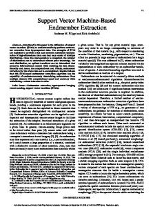
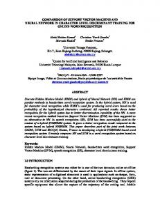
Here, we use one-tailed paired t-test to compare the average total accuracy. Note t-test is just a heuristic method for comparison in here due to the fact that the twenty rates (ten pairs) are not independent. A. Dataset 1 The first dataset is about UK corporations from the Financial Analysis Made Easy (FAME) CD-ROM database which can be found in [1, App.]. It contains 30 failed and 30 nonfailed firms. 12 variables are used as the firms’ characteristics. (01). Sales. (02). ROCE: profit before tax/capital employed (%). (03). FFTL: funds flow (earnings before interest, tax and depreciation)/total liabilities. (04). GEAR: (current liabilities long-term debt)/total assets. (05). CLTA: current liabilities/total assets. (06). CACL: current assets/current liabilities. stock)/current liabili(07). QACL: (current assets ties. (08). WCTA: (current assets current liabilities)/total assets. (09). LAG: number of days between account year end and the date the annual report and accounts were failed at company registry. (10). AGE: number of years the company has been operating since incorporation date. (11). CHAUD: coded 1 if changed auditor in previous three years, 0 otherwise. (12). BIG6: coded 1 if company auditor is a Big6 auditor, 0 otherwise. In each individual test, 40 firms are randomly drawn as the training sample. Due to the scarcity of inputs, we make the number of good firms equal to the number of bad firms in both the training and testing samples, so as to avoid the embarrassing situations that just two or three good (or bad, equally likely) inputs in the test sample. For example the Type1 accuracy can only be 0, 50% or 100% if the test dataset include only two good instances. Thus the test dataset has 10 data of each class. In ANN a two-layer feed-forward network with three TANSIG neurons in the first layer and one PURELIN neuron is used. The network training function is the TRAINLM. In all SVMs, the regularization parameter , for polynomial kernel and for the RBF kernel. The above parameters are obtained by trail and error. Such test is repeated ten times and the final Type1 and type2 accuracy is the average of the results of the ten individual tests. The computational results are shown in the Table I. The column titled Std is the sample standard deviations of ten overall rates from the ten independent tests by the methods specified by the first three columns. The best average test performance is underlined and denoted in bold face. Bold face script is used to tabulate performances that are not significantly lower at the 10% level than the top performance using a two-tailed paired t-test. Other performances are tabulated using normal script. The top three performances are ranked in the last

WANG et al.: A NEW FUZZY SUPPORT VECTOR MACHINE TO EVALUATE CREDIT RISK

827

TABLE I EMPIRICAL RESULTS ON THE DATASET 1

column. The following two empirical tests are also present in the same format. Note Type1 rate, Type2 rate, and overall rate are identical in each pair in Table I. The outcome is due to the fact that the test dataset has ten positive instances and 10 negative instances. The cutoff is selected such that the top 50% instances are labeled as positive and others negative (the 50% is determined by the population of training dataset). If the top ten instances labeled as positive include positive instances, the other 10 instances labeled as negative include - positive instances and - negative instances, so both Type1 rate and Type2 rate are . As shown in the Table I, the new FSVM with RBF kernel and logit regression membership generation achieves the best performance. It correctly classifies 79% of goods instances and 79% of bad firms. The standard SVM with RBF kernel and B-FSVM with RBF kernel and neural network membership achieve the second best performance. Among the 24 methods,

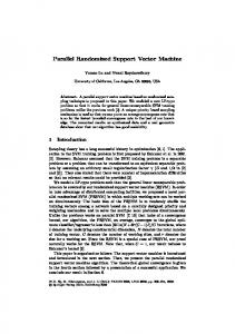
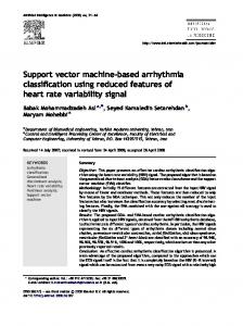
19 methods’ average total classification rates are found lower than the best performance at 10% level by one-tail paired t-test. It is obvious that the B-FSVM is better than U-FSVM in most of the combinations of kernels and membership generating methods. B. Dataset 2 The second dataset is about Japanese credit card application approval obtained UCI Machine Learning Repository. For confidentiality all attribute names and values have been changed to meaningless symbols. After deleting the data with missing attribute values, we obtain 653 data, with 357 cases granted and 296 cases refused. In the 15 attributes, A4–A7 and A13 are multivalue attributes. is a -value attribute, we encode it with 0–1 dummy If variables in linear regression and logit regression and -value (from 1 to ) variables in ANN and SVMs.

828

IEEE TRANSACTIONS ON FUZZY SYSTEMS, VOL. 13, NO. 6, DECEMBER 2005

TABLE II EMPIRICAL RESULTS ON THE DATASET 2

In this empirical test we randomly draw 400 data from the 653 data as the training sample and the else as the test sample. In ANN a two-layer feed-forward network with 4 TANSIG neurons in the first layer and one PURELIN neuron is used. The network training function is the TRAINLM. In all SVMs, the , for polynomial kernel and kernel parameters for the RBF kernel. The previous parameters are obtained by trial and error. Table II summaries the results of comparisons. B-FSVM with polynomial kernel and logistic regression membership generation achieves the best performance. B-FSVM with RBF kernel and logistic regression membership generation and logit regression and achieves the second and third best performance respectively. The average performances of half of the 24 models are found below the best performance at 10% level by one-tailed paired t-test. The results also show that the new fuzzy SVM is better than standard SVM and U-FSVM when they use the same kernel in most cases.

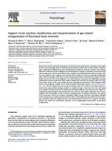
C. Dataset 3 The third dataset is from the CD ROM accessory of [27]. The data set contains 1225 applicants, of which 323 are observed bad creditors. The following 12 variables are chosen in our test. (01). Year of birth. (02). Number of children. (03). Number of other dependents. (04). Is there a home phone (binary). (05). Spouse’s income. (06). Applicant’s income. (07). Value of home. (08). Mortgage balance outstanding. (09). Outgoings on mortgage or rent. (10). Outgoings on loans. (11). Outgoings on hire purchase. (12). Outgoings on credit cards.

WANG et al.: A NEW FUZZY SUPPORT VECTOR MACHINE TO EVALUATE CREDIT RISK

829

TABLE III EMPIRICAL RESULTS ON THE DATASET 3

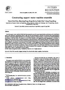
In the dataset, the numbers of healthy cases (902) are nearly three times of delinquent cases (323). To make the numbers of the two classes nearly equal, we triple delinquent data, i.e., means we add two copy of each delinquent case. Thus the total dataset includes 1871 data. Then we randomly draw 800 data from the 1871 data as the training sample and else as the test sample. In ANN a two-layer feed-forward network with four TANSIG neurons in the first layer and one PURELIN neuron is used. The network training function is the TRAINLM. In all support vector machines the regularization parameter is 50. In for polynomial all SVM, the kernel parameters are same, for the RBF kernel. Such trial is repeated ten kernel and times. The results are presented in Table III. It is obvious that the separability of the dataset is clearly lower than the previous two datasets. All models’ average overall classification accuracy is less than 70%. The best performance is achieved by

the B-FSVM with RBF kernel and logistic regression membership generation. B-FSVM with RBF kernel and linear regression membership generation and U-FSVM with RBF and logit regression membership generation achieves the second and third best performances respectively. The lower separability also be can be seem that only 8 models in 24 models are found lower average performance than the best performance at 10% level by one-tail paired t-test. It seems that the average performances of standard SVM, U-FSVM and B-FSVM are quite close in this test. It may be due to the undesirable membership generation. The linear regression, logit regression and ANN themselves only achieves the average overall performances 64.12%, 64.18%, and 62.13%. We believe that bad memberships may provide wrong signals and disturb the training of the SVM, instead of deceasing its vulnerability to outliers in most the combinations of kernels and membership generation methods.

830

IEEE TRANSACTIONS ON FUZZY SYSTEMS, VOL. 13, NO. 6, DECEMBER 2005

V. SUMMARY AND CONCLUSION A. Contributions of This Study This paper presents a bilateral weighted fuzzy SVM in which every applicant in the training dataset is regarded as both good and bad class with different memberships that is generated by some basic credit scoring methods. By this way, we expect the new fuzzy SVM to achieve better generalization ability while keeping the merit of insensitive to outliers as the Unilateral-weighted fuzzy SVM in [11] and [15]. We reformulate the training problem into a quadratic programming problem. To evaluate its applicability and performance in real credit world, three real world datasets are used to compare its classification rate with standard SVM and U-FSVM. The empirical results show that the new fuzzy SVM can find promising application in credit analysis. It can achieve better generalizing result than standard SVM and the fuzzy SVM propose in [11] and [15] in many cases (the combinations of kernel and membership generation methods). The results also show that the new fuzzy SVM can consistently achieve comparable performance than traditional credit scoring methods if it uses RBF kernel and the memberships generated by logistic regression. It achieves the best average performance in dataset 1 and dataset 3 and second best in dataset 2. Moreover in empirical test 1 and 2, the performance of B-FSVM is better than standard SVM and U-FSVM for many combinations of kernels and membership generation methods. B. Limitations and Implications for Researchers and Practitioners Though the empirical tests on three datasets show that the new fuzzy SVM is promising, the study reported here is far from sufficient to generate any conclusive statements about the performance of our new fuzzy SVM in general. Since the positive performances depends on the characteristics of the datasets, further research are encouraged to apply the new fuzzy SVM to credit analysis to determine whether our new fuzzy support vector machine can indeed have superior results as shown in our comparisons in this paper. Comparing overall classification rates in the three datasets, we can clearly see that their performances vary a dataset from another. Especially the average performance of B-FSVM with polynomial kernel and logit regression membership generation achieves the best performance in empirical test 2, while the second worst in empirical test. So the kernel and membership generation method must be chosen appropriately when apply the new fuzzy SVM method to credit scoring. Furthermore, there are several limitations that may restrict the use of neural network models for its applications. Membership generation: The performance of fuzzy SVM highly depends on the discriminatory power of the membership generation method. Undesirable memberships will sent wrong messages to the training process and disturb the training instead. Such “rubbish-in-rubbish-out” suggests that in application we should check the efficiency of membership generation methods before solving the quadratic programming (33). In some unfavorable cases, we may have to discard the new SVM and resort to the standard SVM.

Computational complexity: Another major issue of our new fuzzy SVM method is the computational complexity. For a training dataset with data, our new model needs to solve a quadratic programming problem, compared with a -dimension quadratic programming problem in standard SVM and U-FSVM. It takes half a minute on average to complete training of SVM and U-FSVM and 2.5 minutes on average to complete the B-FSVM in empirical test 2, in which the training dataset include 400 instances. It takes 3 minutes on average to complete training of SVM and U-FSVM and 45 minutes to complete the B-FSVM in empirical test 3, in which the training dataset includes 800 instances. Compared with the SVMs, linear regression and logit regression takes less than 10 second and ANN takes less than half minute in all tests. All the above training runs on a computer with CPU 1.8G. Because sometimes the training is based on a massive dataset, maybe 50 000–100 000 cases, the computational complexity involved in solving such high-dimensional quadratic programming seems to be a major issue in its application. We must tradeoff the discriminatory power and computational effort. REFERENCES [1] M. J. Beynon and M. J. Peel, “Variable precision rough set theory and data discretization: An application to corporate failure prediction,” Omega, vol. 29, pp. 561–576, 2001. [2] S. Chatterjee and S. Barcun, “A nonparametric approach to credit screening,” J. Amer. Statist. Assoc., vol. 65, pp. 50–154, 1970. [3] M. C. Chen and S. H. Huang, “Credit scoring and rejected instances reassigning through evolutionary computation techniques,” Expert Syst. Appl., vol. 24, pp. 433–441, May 2003. [4] Y. C. Coffman, The Proper Role of Tree Analysis in Forecasting the Risk Behavior of Borrowers, MDC Reports. Atlanta, GA: Management Decision Systems, 1986. [5] A. I. Dimitras, R. Slowinski, R. Susmaga, and C. Zopounidis, “Business failure prediction using rough sets,” Eur. J. Oper. Res., vol. 114, pp. 263–290, Apr. 1999. [6] R. A. Fisher, “The use of multiple measurements in taxonomic problems,” Ann. Eugenics, vol. 7, pp. 179–188, 1936. [7] F. Glover, “Improved linear programming models for discriminant analysis,” Decision Sci., vol. 21, pp. 771–785, 1990. [8] B. J. Grablowsky and W. K. Talley, “Probit and discriminant functions for classifying credit applicants: A comparison,” J. Econ. Bus., vol. 33, pp. 254–261, 1981. [9] I. Guyon, N. Matic´ , and V. N. Vapnik, Discovering Information Patterns and Data Cleaning. Cambridge, MA: MIT Press, 1996. [10] W. E. Henley and D. J. Hand, “A k-NN classifier for assessing consumer credit risk,” Statistician, vol. 45, pp. 77–95, Jan. 1996. [11] H. P. Huang and Y. H. Liu, “Fuzzy support vector machines for pattern recognition and data mining,” Int. J. Fuzzy Syst., vol. 4, pp. 826–835, Sep. 2002. [12] Z. Huang, H. C. Chen, C. J. Hsu, W. H. Chen, and S. S. Wu, “Credit rating analysis with support vector machines and neural networks: A market comparative study,” Decision Support Systems, to be published. [13] J. T. Kwok, “The evidence framework applied to support vector machines,” Neural Comput., vol. 11, pp. 1162–1173. [14] T. S. Lee, C. C. Chiu, C. J. Lu, and I. F. Chen, “Credit scoring using the hybrid neural discriminant technique,” Expert Syst. Appl., vol. 23, pp. 245–254, Oct. 2002. [15] C. F. Lin and S. D. Wang, “Fuzzy support vector machine,” IEEE Trans. Neural Netw., vol. 13, no. 2, pp. 464–471, Mar. 2002. [16] P. Makowski, “Credit scoring branches out,” Credit World, vol. 75, pp. 30–37, 1985. [17] R. Malhotra and D. K. Malhotra, “Evaluating consumer loans using neural networks,” Omega, vol. 31, pp. 83–96, Apr. 2003. [18] , “Differentiating between good credits and bad credits using neurofuzzy systems,” Eur. J. Oper. Res., vol. 136, pp. 190–211, Jan. 2002. [19] O. L. Mangasarian, “Linear and nonlinear separation of patterns by linear programming,” Oper. Res. , vol. 13, pp. 444–452, May/Jan. 1965.

WANG et al.: A NEW FUZZY SUPPORT VECTOR MACHINE TO EVALUATE CREDIT RISK

[20] Z. Pawlak, “Rough sets,” Int. J. Comput. Inform. Sci., vol. 11, pp. 341–356, 1982. [21] S. Piramuthu, “Financial credit-risk evaluation with neural and neurofuzzy systems,” Eur. J. Oper. Res., vol. 112, pp. 310–321, Jan. 1999. [22] R. Smalz and M. Conrad, “Combining evolution with credit apportionment: A new learning algorithm for neural nets,” Neural Networks, vol. 7, pp. 341–351, 1994. [23] R. Stecking and K. B. Schebesch, “Support vector machines for credit scoring: Comparing to and combining with some traditional classification methods,” in Between Data Science and Applied Data Analysis, M. Schader, W. Gaul, and M. Vichy, Eds. Berlin, Germany: SpringerVerlag, 2003, pp. 604–612. [24] J. A. K. Suykens, J. De Brabanter, L. Lukas, and J. Vandewalle, “Weighted least squares support vector machine: Robustness and sparse approximation,” Neurocomput., vol. 48, pp. 85–105, 2002. [25] J. A. K. Suykens and J. V. Vandewalle, “Least squares support vector machine classifiers,” Neural Process. Lett., vol. 9, pp. 293–300, Jun. 1999. [26] J. A. K. Suykens, T. Van Gestel, J. De Brabanter, B. De Moor, and J. Vandewalle, Least Squares Support Vector Machines. Singapore: World Scientific, 2002. [27] L. C. Thomas, “A survey of credit and behavioral scoring: Forecasting financial risk of lending to consumers,” Int. J. Forecasting, vol. 16, pp. 149–172, Apr.–Jun. 2002. [28] L. C. Thomas, D. B. Edelman, and J. N. Crook, Credit Scoring and its Applications. Philadelphia, PA: SIAM, 2002. [29] D. Tsujinishi and S. Abe, “Fuzzy least squares support vector machines for multiclass problems,” Nerual Networks, vol. 16, pp. 785–792, 2003. [30] T. Van Gestel, B. Baesens, J. Garcia, and P. Van Dijcke, “A support vector machine approach to credit scoring,” Bank en Financiewezen, vol. 2, pp. 73–82, 2003. [31] T. Van Gestel, B. Baesens, J. A. K. Suykens, M. De Espinoza, J. Baestaens, De Vanthienen, and B. Moor, “Bankruptcy prediction with least squares support vector machine classifiers,” in Proc. IEEE Int. Conf. Computational Intelligence for Financial Engineering, Hong Kong, 2003. [32] T. Van Gestel, J. A. K. Suykens, G. Lanckriet, A. Lambrechts, B. De Moor, and J. Vandewalle, “Bayesian framework for least squares support vector machine classifiers, Gaussian processes and kernel Fisher discriminant analysis,” Neural Comput., vol. 15, no. 5, pp. 1115–1148, 2002. [33] V. Vapnik, The Nature of Statistical Learning Theory. New York: Springer, 1995. , Statistical Learning Theory. New York: Wiley, 1998. [34] , “The support vector method of function estimation,” in Nonlinear [35] Modeling: Advanced Black-Box Techniques, J. A. K. Suykensand and J. Vandewale, Eds. Boston, MA: Kluwer, 1998, pp. 55–85. [36] F. Varetto, “Genetic algorithms applications in the analysis of insolvency risk,” J. Banking Finance, vol. 22, pp. 1421–1439, Oct. 1998. [37] D. West, “Neural network credit scoring models,” Comput. Oper. Res., vol. 27, pp. 1131–1152, Sep. 2000.

831

[38] J. C. Wiginton, “A note on the comparison of logit and discriminant models of consumer credit behavior,” J. Financial Quant. Anal., vol. 15, pp. 757–770, Sep. 1980. [39] X. Zhang, “Using class-center vectors to build support vector machines,” in Proc. IEEE NNSP, 1999, pp. 3–11.

Yongqiao Wang is currently working toward the Ph.D. degree at the Institute of Systems Science, Chinese Academy of Sciences (CAS), Beijing, China. His current research interests include credit risk analysis, financial engineering, and data mining.

Shouyang Wang received the Ph.D. degree in operations research from the Institute of Systems Science, Chinese Academy of Sciences (CAS), Beijing, China, in 1986. He is currently a Bairen Distinguished Professor of Management Science at the Academy of Mathematics and Systems Sciences of CAS and a Lotus Chair Professor at Hunan University, Changsha, China. He is the editor-in-chief or a co-editor of 12 journals. He has published 18 books and over 120 journal papers. His current research interests include financial engineering, e-auctions, and decision support systems.

K. K. Lai received the Ph.D. degree from Michigan State University, East Lansing. He is the Chair Professor of Management Sciences at City University of Hong Kong and the Associate Dean of the Faculty of Business. Prior to his current post, he was an Operational Research Analyst at Cathay Pacific Airways and an Area Manager on Marketing Information Systems at Union Carbide Eastern. His main areas of research interests are logistics and operations management, computer simulation, and business decision modeling.