Using the Support Vector Machine as a. Classification Method for Software Defect. Prediction with Static Code Metrics. David Gray, David Bowes, Neil Davey, ...
Using the Support Vector Machine as a Classification Method for Software Defect Prediction with Static Code Metrics David Gray, David Bowes, Neil Davey, Yi Sun and Bruce Christianson Science and Technology Research Institute, University of Hertfordshire, UK (d.gray, d.h.bowes, n.davey, y.2.sun, b.christianson)@herts.ac.uk
Abstract. The automated detection of defective modules within software systems could lead to reduced development costs and more reliable software. In this work the static code metrics for a collection of modules contained within eleven NASA data sets are used with a Support Vector Machine classifier. A rigorous sequence of pre-processing steps were applied to the data prior to classification, including the balancing of both classes (defective or otherwise) and the removal of a large number of repeating instances. The Support Vector Machine in this experiment yields an average accuracy of 70% on previously unseen data.
1
Introduction
oftware defect prediction is the process of locating defective modules in S software and is currently a very active area of research within the software engineering community. This is understandable as “Faulty software costs businesses $78 billion per year” ([1], published in 2001), therefore any attempt to reduce the number of latent defects that remain inside a deployed system is a worthwhile endeavour. Thus the aim of this study is to observe the classification performance of the Support Vector Machine (SVM) for defect prediction in the context of eleven data sets from the NASA Metrics Data Program (MDP) repository; a collection of data sets generated from NASA software systems and intended for defect prediction research. Although defect prediction studies have been carried out with these data sets and various classifiers (including an SVM) in the past, this study is novel in that thorough data cleansing methods are used explicitly. The main purpose of static code metrics (examples of which include the number of: lines of code, operators (as proposed in [2]) and linearly independent paths (as proposed in [3]) in a module) is to give software project managers an indication toward the quality of a software system. Although the individual worth of such metrics has been questioned by many authors within the software engineering community (see [4], [5], [6]), they still continue to be used. Data mining techniques from the field of artificial intelligence now make it possible to predict software defects; undesired outputs or effects produced by
software, from static code metrics. Views toward the worth of using such metrics for defect prediction are as varied within the software engineering community as those toward the worth of static code metrics. However, the findings within this paper suggest that such predictors are useful, as on the data used in this study they predict defective modules with an average accuracy of 70%.
2 2.1
Background Static Code Metrics
Static code metrics are measurements of software features that may potentially relate to quality. Examples of such features and how they are often measured include: size, via lines of code (LOC) counts; readability, via operand and operator counts (as proposed by [2]) and complexity, via independent path counts (as proposed by [3]). Because static code metrics are calculated through the parsing of source code their collection can be automated. Thus it is computationally feasible to calculate the metrics of entire software systems, irrespective of their size. [7] points out that such collections of metrics can be used in the following contexts: – To make general predictions about a system as a whole. For example, has a system reached a required quality threshold? – To identify anomalous components. Of all the modules within a software system, which ones exhibit characteristics that deviate from the overall average? Modules highlighted as such can then be used as pointers to where developers should be focusing their efforts. [8] points out that this is common practice amongst several large US government contractors. 2.2
The Support Vector Machine
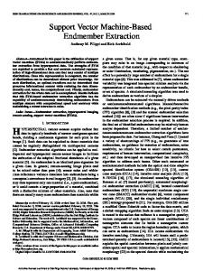
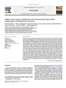
A Support Vector Machine (SVM) is a supervised machine learning algorithm that can be used for both classification and regression [9]. SVMs are known as maximum margin classifiers as they find the best separating hyperplane between two classes (see Fig. 1). This process can also be applied recursively to allow the separation of any number of classes. Only those data points that are located nearest to this dividing hyperplane, known as the support vectors, are used by the classifier. This enables SVMs to be used successfully with both large and small data sets. Although maximum margin classifiers are strictly intended for linear classification, they can also be used successfully for non-linear classification (such as the case here) via the use of a kernel function. A kernel function is used to implicitly map the data points into a higher-dimensional feature space, and to take the inner-product in that feature space [10]. The benefit of using a kernel function is that the data is more likely to be linearly separable in the higher feature space. Additionally, the actual mapping to the higher-dimensional space is never needed.
There are a number of different kinds of kernel functions (any continuous symmetric positive semi-definite function will suffice) including: linear, polynomial, Gaussian and sigmoidal. Each have varying characteristics and are suitable for different problem domains. The one used here is the Gaussian radial basis function (RBF), as it can handle non-linear problems, requires fewer parameters than other non-linear kernels and is computationally less demanding than the polynomial kernel [11].
Fig. 1. A binary classification toy problem: separate dots from triangles. The solid line shows the optimal hyperplane. The dashed lines parallel to the solid one show how much one can move the decision hyperplane without misclassification.
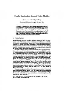
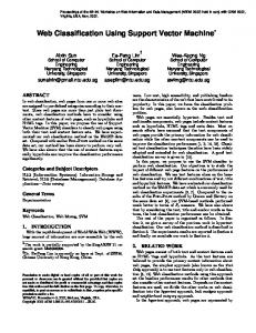
When an SVM is used with a Gaussian RBF kernel, there are two userspecified parameters, C and γ. C is the error cost parameter; a variable that determines the trade-off between minimising the training error and maximizing
the margin (see Fig. 2). γ controls the width / radius of the Gaussian RBF. The performance of an SVM is largely dependant on these parameters, and the optimal values need to be determined for each training set via a systematic search.
Fig. 2. The importance of optimal parameter selection. The solid and hollow dots represent the training data for two classes. The hollow dot with a dot inside is the test data. Observe that the test dot will be misclassified if too simple (underfitting, the straight line) or too complex (overfitting, the jagged line) a hyperplane is chosen. The optimum hyperplane is shown by the oval line.
2.3
Data
The data used within this study was obtained from the NASA Metrics Data Program (MDP) repository1 . This repository currently contains thirteen data sets, each of which represent a NASA software system / subsystem and contain the static code metrics and corresponding fault data for each comprising module. Note that a module in this domain can refer to a function, procedure or method. Eleven of these thirteen data sets were used in this study: brief details of each are shown in Table 1. A total of 42 metrics and a unique module identifier comprise each data set (see Table 5, located in the appendix), with the exception of MC1 and PC5 which do not contain the decision density metric. 1
http://mdp.ivv.nasa.gov/
Table 1. The eleven NASA MDP data sets that were used in this study. Note that KLOC refers to thousand lines of code. Name
Language
Total KLOC
No. of Modules
% Defective Modules
CM1
C
20
505
10
KC3 KC4
Java Perl
18 25
458 125
9 49
MC1 MC2
C & C++ C
63 6
9466 161
0.7 32
MW1
C
8
403
8
40 26 40 36 164
1107 5589 1563 1458 17168
7 0.4 10 12 3
PC1 PC2 PC3 PC4 PC5
C C++
All the metrics shown within Table 5 with the exception of error count and error density, were generated using McCabeIQ 7.1; a commercial tool for the automated collection of static code metrics. The error count metric was calculated by the number of error reports that were issued for each module via a bug tracking system. Each error report increments the value by one. Error density is derived from error count and LOC total, and describes the number of errors per thousand LOC (KLOC).
3 3.1
Method Data Pre-processing
The process for cleansing each of the data sets used in this study is as follows: Initial Data Set Modifications Each of the data sets initially had their module identifier and error density attribute removed, as these are not required for classification. The error count attribute was then converted into a binary target attribute for each instance by assigning all values greater than zero to defective, non-defective otherwise. Removing Repeated and Inconsistent Instances Repeated feature vectors, whether with the same (repeated instances) or different (inconsistent instances) class labels, are a known problem within the data mining community [12]. Ensuring that training and testing sets do not share instances guarantees that all classifiers are being tested against previously unseen data. This is very
important as testing a predictor upon the data used to train it can greatly overestimate performance [12]. The removal of inconsistent items from training data is also important, as it is clearly illogical in the context of binary classification for a classifier to associate the same data point with both classes. Carrying out this pre-processing stage showed that some data sets (namely MC1, PC2 and PC5) had an overwhelmingly high number of repeating instances (79%, 75% and 90% respectively, see Table 2). Although no explanation has yet been found for these high number of repeated instances, it appears highly unlikely that this is a true representation of the data, i.e. that 90% of modules within a system / subsystem could possibly have the same number of: lines, comments, operands, operators, unique operands, unique operators, conditional statements, etc. Table 2. The result of removing all repeated and inconsistent instances from the data. Name
Original Instances
Instances Removed
% Removed
CM1
505
51
10
KC3
458
134
29
KC4
125
12
10
MC1
9466
7470
79
MC2
161
5
3
MW1
403
27
7
PC1
1107
158
14
PC2
5589
4187
75
PC3
1563
130
8
PC4
1458
116
8
PC5
17186
15382
90
Total
38021
27672
73
Removing Constant Attributes If an attribute has a fixed value throughout all instances then it is obviously of no use to a classifier and should be removed. Each data set had between 1 and 4 attributes removed during this phase with the exception of KC4 that had a total of 26. Details are not shown here due to space limitations. Missing Values Missing values are those that are unintentionally or otherwise absent for a particular attribute in a particular instance of a data set. The only missing values within the data sets used in this study were within the decision density attribute of data sets CM1, KC3, MC2, MW1, PC1, PC2, and PC3.
Manual inspection of these missing values indicated that they were almost certainly supposed to be representing zero, and were replaced accordingly. Balancing the Data All the data sets used within this study, with the exception of KC4, contain a much larger amount of one class (namely, non-defective) than they do the other. When such imbalanced data is used with a supervised classification algorithm such as an SVM, the classifier will be expected to over predict the majority class [10], as this will produce lower error rates in the test set. There are various techniques that can be used to balance data (see [13]). The approach taken here is the simplest however, and involves randomly undersampling the majority class until it becomes equal in size to that of the minority class. The number of instances that were removed during this undersampling process, along with the final number of instances contained within each data set, are shown in Table 3.
Table 3. The result of balancing each data set. Name
Instances Removed
% Removed
Final no. of Instances
CM1
362
80
92
KC3
240
74
84
KC4
1
1
112
MC1
1924
96
72
MC2
54
35
102
MW1
320
85
56
PC1
823
87
126
PC2
1360
97
42
PC3
1133
79
300
PC4
990
74
352
PC5
862
48
942
Normalisation All values within the data sets used in this study are numeric, so to prevent attributes with a large range dominating the classification model all values were normalised between -1 and +1. Note that this pre-processing stage was performed just prior to training for each training and testing set, and that each training / testing set pair were scaled in the same manner [11].
Randomising Instance Order The order of the instances within each data set were randomised to defend against order effects, where the performance of a predictor fluctuates due to certain orderings within the data [14].
3.2
Experimental Design
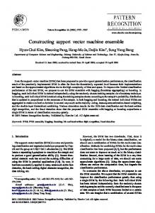
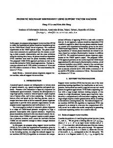
When splitting each of the data sets into training and testing sets it is important to ameliorate possible anomalous results. To this end we use five-fold crossvalidation. Note that to reduce the effects of sampling bias introduced when randomly splitting each data set into five bins, the cross-validation process was repeated 10 times for each data set in each iteration of the experiment (described below). As mentioned in Section 2.2, an SVM with an RBF kernel requires the selection of optimal values for parameters C and γ for maximal performance. Both values were chosen for each training set using a five-fold grid search (see [11]), a process that uses cross-validation and a wide range of possible parameter values in a systematic fashion. The pair of values that yield the highest average accuracy are then taken as the optimal parameters and used when generating the final model for classification. Due to the high percentage of information lost when balancing each data set (with the exception of KC4), the experiment is repeated fifty times. This is in order to further minimise the effects of sampling bias introduced by the random undersampling that takes place during balancing. Pseudocode for the full experiment carried out in this study is shown in Fig 3. Our chosen SVM environment is LIBSVM [15], an open source library for SVM experimentation.
Fig. 3. Pseudocode for the experiment carried out in this study. M = 50 N = 10 V = 5
# No. of times to repeat full experiment # No. of cross-validation repetitions # No. of cross-validation folds
DATASETS = ( CM1, KC3, KC4, MC1, MC2, MW1, PC1, PC2, PC3, PC4, PC5 ) results = ( )
# An empty list
repeat M times: for dataSet in DATASETS: dataSet = pre_process(dataSet) # As described in Section 3.1 repeat N times: for i in 1 to V: testerSet = dataSet[i] trainingSet = dataSet - testerSet params = gridSearch(trainingSet) model = svm_train(params, trainingSet) results += svm_predict(model, testerSet) FinalResults = avg(results)
4
Assessing Performance
The measure used to assess predictor performance in this study is accuracy. Accuracy is defined as the ratio of instances correctly classified out of the total number of instances. Although simple, accuracy is a suitable performance measure for this study as each test set is balanced. For imbalanced test sets more complicated measures are required.
5
Results
The average results for each data set are shown in Table 4. The results show an average accuracy of 70% across all 11 data sets, with a range of 64% to 82%. Notice that there is a fairly high deviation shown within the results. This is to be expected due to the large amount of data lost during balancing and supports the decision for the experiment being repeated fifty times (see Fig. 3). It is notable that the accuracy for some data sets is extremely high, for example with data set PC4, four out of every five modules were being correctly classified. The results show that all data sets with the exception of PC2 have a mean accuracy greater than two standard deviations away from 50%. This shows the statistical significance of the classification results when compared to a dumb classifier that predicts all one class (and therefore scores an accuracy of 50%).
Table 4. The results obtained from this study. Name
% Mean Accuracy
Std.
CM1
68
5.57
KC3
66
6.56
KC4
71
4.93
MC1
65
6.74
MC2
64
5.68
MW1
71
7.3
PC1
71
5.15
PC2
64
9.17
PC3
76
2.15
PC4
82
2.11
PC5
69
1.41
Total
70
5.16
6
Analysis
Previous studies ([16], [17], [18]) have also used data from the NASA MDP repository and an SVM classifier. Some of these studies briefly mention data pre-processing, however we believe that it is important to explicitly carry out all of the data cleansing stages described here. This is especially true with regard to the removal of repeating instances, ensuring that all classifiers are being tested against previously unseen data. The high number of repeating instances found within the MDP data sets was surprising. Brief analysis of other defect prediction data sets showed a repeating average of just 1.4%. We are therefore suspicious of the suitability of the data held within the MDP repository for defect prediction and believe that previous studies which have used this data and not carried out appropriate data cleansing methods may be reporting inflated performance values. An example of such a study is [18], where the authors use an SVM and four of the NASA data sets, three of which were used in this study (namely CM1, PC1 and KC3). The authors make no mention of data pre-processing other than the use of an attribute selection algorithm. They then go on to report a minimum average precision, the ratio of correctly predicted defective modules to the total number of defective modules, of 84.95% and a minimum average recall, the ratio of defective modules detected as such, of 99.4%. We believe that such high classification rates are highly unlikely in this problem domain due to the limitations of static code metrics and that not carrying out appropriate data cleansing methods may have been a factor in these high results.
7
Conclusion
This study has shown that on the data studied here the Support Vector Machine can be used successfully as a classification method for defect prediction. We hope to improve upon these results in the near future however via the use of a oneclass SVM; an extension to the original SVM algorithm that trains upon only defective examples, or a more sophisticated balancing technique such as SMOTE (Synthetic Minority Over-sampling Technique). Our results also show that previous studies which have used the NASA data may have exaggerated the predictive power of static code metrics. If this is not the case then we would recommend the explicit documentation of what data pre-processing methods have been applied. Static code metrics can only be used as probabilistic statements toward the quality of a module and further research may need to be undertaken to define a new set of metrics specifically designed for defect prediction. The importance of data analysis and data quality has been highlighted in this study, especially with regard to the high quantity of repeated instances found within a number of the data sets. The issue of data quality is very important within any data mining experiment as poor quality data can threaten the validity of both the results and the conclusions drawn from them [19].
8
Appendix Table 5. The 42 metrics originally found within each data set. Metric Type
Metric Name
McCabe
01. 02. 03. 04. 05. 06. 07. 08. 09. 10. 11. 12.
Cyclomatic Complexity Cyclomatic Density Decision Density Design Density Essential Complexity Essential Density Global Data Density Global Data Complexity Maintenance Severity Module Design Complexity Pathological Complexity Normalised Cyclomatic Complexity
Raw Halstead
13. 14. 15. 16.
Number Number Number Number
Derived Halstead
17. 18. 19. 20. 21. 22. 23. 24.
Length (N) Volume (V) Level (L) Difficulty (D) Intellegent Content (I) Programming Effort (E) Error Estimate (B) Programming Time (T)
25. 26. 27. 28. 29. 30.
LOC Total LOC Executable LOC Comments LOC Code and Comments LOC Blank Number of Lines (opening to closing bracket)
Misc.
31. 32. 33. 34. 35. 36. 37. 38. 39. 40.
Node Count Edge Count Branch Count Condition Count Decision Count Formal Parameter Count Modified Condition Count Multiple Condition Count Call Pairs Percent Comments
Error
41. Error Count 42. Error Density
LOC Counts
of of of of
Operators Operands Unique Operators Unique Operands
References 1. Levinson, M.: Lets stop wasting $78 billion per year. CIO Magazine (2001) 2. Halstead, M.H.: Elements of Software Science (Operating and programming systems series). Elsevier Science Inc., New York, NY, USA (1977) 3. McCabe, T.J.: A complexity measure. In: ICSE ’76: Proceedings of the 2nd international conference on Software engineering, Los Alamitos, CA, USA, IEEE Computer Society Press (1976) 407 4. Hamer, P.G., Frewin, G.D.: M.H. Halstead’s Software Science - a critical examination. In: ICSE ’82: Proceedings of the 6th international conference on Software engineering, Los Alamitos, CA, USA, IEEE Computer Society Press (1982) 197– 206 5. Shen, V.Y., Conte, S.D., Dunsmore, H.E.: Software Science Revisited: A critical analysis of the theory and its empirical support. IEEE Trans. Softw. Eng. 9(2) (1983) 155–165 6. Shepperd, M.: A critique of cyclomatic complexity as a software metric. Softw. Eng. J. 3(2) (1988) 30–36 7. Sommerville, I.: Software Engineering: (8th Edition) (International Computer Science Series). Addison Wesley (2006) 8. Menzies, T., Greenwald, J., Frank, A.: Data mining static code attributes to learn defect predictors. Software Engineering, IEEE Transactions on 33(1) (Jan. 2007) 2–13 9. Sch¨ olkopf, B., Smola, A.J.: Learning with Kernels: Support Vector Machines, Regularization, Optimization, and Beyond (Adaptive Computation and Machine Learning). The MIT Press (2001) 10. Sun, Y., Robinson, M., Adams, R., Boekhorst, R.T., Rust, A.G., Davey, N.: Using sampling methods to improve binding site predictions. In: Proceedings of ESANN. (2006) 11. Hsu, C.W., Chang, C.C., Lin, C.J.: A practical guide to support vector classification. Technical report, Taipei (2003) 12. Witten, I.H., Frank, E.: Data Mining: Practical Machine Learning Tools and Techniques. Second edn. Morgan Kaufmann Series in Data Management Systems. Morgan Kaufmann (June 2005) 13. Wu, G., Chang, E.Y.: Class-boundary alignment for imbalanced dataset learning. In: ICML 2003 Workshop on Learning from Imbalanced Data Sets. (2003) 49–56 14. Fisher, D.: Ordering effects in incremental learning. In: Proc. of the 1993 AAAI Spring Symposium on Training Issues in Incremental Learning, Stanford, California (1993) 34–41 15. Chang, C.C., Lin, C.J.: LIBSVM: a library for support vector machines. (2001) Software available at http://www.csie.ntu.edu.tw/∼cjlin/libsvm. 16. Li, Z., Reformat, M.: A practical method for the software fault-prediction. Information Reuse and Integration, 2007. IRI 2007. IEEE International Conference on (Aug. 2007) 659–666 17. Lessmann, S., Baesens, B., Mues, C., Pietsch, S.: Benchmarking classification models for software defect prediction: A proposed framework and novel findings. Software Engineering, IEEE Transactions on 34(4) (2008) 485–496 18. Elish, K.O., Elish, M.O.: Predicting defect-prone software modules using support vector machines. J. Syst. Softw. 81(5) (2008) 649–660 19. Liebchen, G.A., Shepperd, M.: Data sets and data quality in software engineering. In: PROMISE ’08: Proceedings of the 4th international workshop on Predictor models in software engineering, New York, NY, USA, ACM (2008) 39–44