A New Methodology for Self Localization in Wireless Sensor Networks

A New Methodology for Self Localization in Wireless Sensor Networks Allon Rai, Sangita Ale, and Syed S. Rizvi

Aasia Riasat

Computer Science and Engineering Department University of Bridgeport Bridgeport, CT USA {Allonrai, Sale, Srizvi}@bridgeport.edu

Computer Science Department Institute of Business Management Karachi, Pakistan [email protected]

Abstract— With the tremendous applications of the wireless sensor network, self-localization has become one of the challenging subject matter that has gained attention of many researchers in the field of wireless sensor network. Localization is the process of assigning or computing the location of the sensor nodes in a sensor network. As the sensor nodes are deployed randomly we do not have any knowledge about their location in advance. As a result, this becomes very important that they localize themselves as manual deployment of sensor node is not feasible. Also, in WSN the main problem is the power as the sensor nodes have very limited power source. So, in this paper, we provide a novel solution for localizing the sensor nodes using controlled power of the beacon nodes such that we will have longer life of the beacon nodes which plays a vital role in the process of localization as it is the only special nodes that has the information about its location when they are deployed such that the remaining ordinary nodes can localize themselves in accordance with these beacon node. We develop a novel model that first finds the distance of the sensor nodes then it finds the location of the unknown sensor nodes in power efficient manner. Our simulation results show the effectiveness of the proposed methodology in terms of controlled and reduced power. Keywords- sensor nodes, localization, scaling, multi-path fading, AoA, TDoA, MDS, WSN

I.

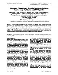
will in turn hamper the network. So this has become one of the main problems in the localization process. As manual localization is not feasible for large sensor network, these nodes has to localize themselves in such a way that they can remain active for a longer period of time such that WSN can function properly for desired period of time. Fig. 1 and Fig. 4 shows a sensor network and also shows how sensor nodes convey the information after their localization (Fig.1). These nodes can be either data originator or data router. The problem of localization has become the matter of interest as sensor nodes need to know their location in the sensor network in order to communicate and relay information to other neighboring sensor nodes as shown in Fig.1. Global Positioning System (GPS) is one of the solutions for this purpose but it is not applicable for large scale sensor network as it is expensive compared to common sensor nodes [3]. Moreover, GPS is limited to outdoor applications only as they are based on satellite communication. Many algorithms have been proposed for localization, but only those algorithms can be implemented that has self managing capability, ability to handle the node failure and range errors and takes into consideration the fact that power is of utmost importance when it comes to wireless sensor network as sensor nodes have a very limited amount of energy resources. Keeping these things

INTRODUCTION

Wireless sensor network (WSN) is one of the growing issues in the field of wireless communication. Such sensor network consists of large number of sensor node having self organizing and computing capability. In various applications such as environmental monitoring, (e.g monitoring volcano activities), hard to reach areas such as natural disasters like earthquake and also in the battle fields, sensor nodes are deployed randomly as shown in Fig 1 and 4.a to get valuable information. Because of their random deployment, it is very necessary that they self localize themselves since the premature knowledge of their location is not possible in large sensor network. Thus, the concept of self localization came into existence and has become the area of great concern for the researchers. The other aspect of localization that has lured the researchers is the minimum power resource of these sensor nodes. All these sensor nodes have battery and radio so as soon as the battery is dead the sensor node is also dead which

Fig 1:Showing sensor network

in mind, in this paper we present a solution to find the location of the sensor nodes using controlled power. In this paper, we have described an algorithm/method of calculating the location of sensor nodes which consists of mainly two parts. The first part is concerned with the evaluation of the distance of the sensor nodes in accordance with the beacon nodes and the second part is concerned with estimation of the location of the sensor nodes in the sensor network. In our model we have given emphasis to the fact that sensor nodes have limited power, and hence the localization has to be done accordingly. II.

METHODS OF SENSOR NODES LOCALIZATION

Localization has allured many researchers in the field of wireless communication. Since localization is one of the biggest challenges that one has to face in the wireless sensor network, many researches has been done and many are still going on. But still there are areas for improvement such as effective power management of the sensor nodes. Using GPS seemed to be the one of the solution to sort out the localization problem but it was not feasible for large sensor network as it is expensive and is not applicable for indoor applications. Here, we are listing some of the pre-existing methodology for the localization of the sensor nodes. The RSSI model is based on the principle that signal strength diminishes with distance [1]. Thus, the distance between the source and the receiver could be found out by the strength of the radio signal received. Here, d is the distance between the transmitter and the receiver, Pr is the received power, and Pt is the transmitted power. The demerits of RSSI method is that it is easily affected by multi-path fading, shadowing, scattering and also in the non line of sight condition. The time difference of arrival method (TDoA) was also devised to calculate the distance of the sensor nodes [10]. This method used extra speaker and a microphone. The sender node sends the radio signal at first and after some time it again sends a sound ‘chirp’. The receiver then detects the radio signal at time tr and the sound at time ts after some time delay td. It then uses this information to calculate the distance between the source node and the destination node.

Here, d is the distance between the source and the receiver, Sr is the radio signal, Ss is the sound. This method was inconvenient because the sensor nodes required an extra microphone and speaker to be built in. The signal speed is also affected by humidity and temperature and for some condition the line of sight is difficult to meet. The radio hop count method used the hop count to find the distance between the sensors nodes, [3]. Hop count is the shortest path between the two nodes. Fig.1 shows the hop count method. Mathematically, this can be expressed as: D = (Avg hop distance X no of hops) where D is the distance between the nodes a and b. The disadvantage of this method is that it results in error of about 0.5R per measurement where R is the maximum range of the radio. The Angle of Arrival (AoA) method was proposed to calculate the distance of the sensor nodes [11]. This method

used Radio and microphone arrays to calculate the distance. In this method, microphones hear the transmitted signal and analyze the phase or the time difference of the arriving signals at the microphone and then calculate the angle of the arriving signal. The demerit of this method is that the hardware used is expensive and bulky compared to TDoA. Moreover, this method is affected by the multi-path effects, shadowing, scattering and also when there is no line of sight condition. Optimization algorithm was proposed for constraint-based localization scheme [11]. In this method, the feasible nodes were constrained by the data (RF communication, angular information) obtained from the optical device. Thus, SemiDefinite programming was used in finding the solution for the optimization problem. For a centralized robust localization algorithm, Multidimensional Scaling (MDS) was proposed, which was a data analysis technique that displayed the data as a geometric picture [13]. Since it required the distance between all the nodes, distributed approach was proposed again that used parallelism and inter node communication to run the network. III.

AN IMPROVED METHODOLOGY FOR CALCULATING DISTANCE AND LOCATION OF SENSOR NODES

As it has already been stated above that the algorithms that are proposed for the localization must be energy efficient. After thorough research we have come up with a solution for this problem. Our model tries to find the location of the sensor nodes by saving the power of the nodes by controlling the amount of power that it requires to transmit the information. Thus our method is divided into two sections: a) distance calculation and b) location calculation In our model, we control the transmission power of the beacon nodes such that we can conserve the energy of the beacon nodes as shown in Fig.2. When the nodes are deployed these beacon nodes are the only nodes that have the information regarding their location in the network and the other ordinary nodes find their location in accordance with the beacon nodes. The main objective of our model is to conserve the power of the beacon nodes and hence find the location of these randomly deployed sensor nodes.

Fig 2. Showing the range of beacon nodes

A. Distance Calculation Beacon nodes in a sensor network are the only special nodes that have the information about their location after they have been randomly deployed in the targeted area where as the other sensor nodes don’t. They rely on the beacon nodes to find their location. Since all the nodes have radio within, what we do is that we control the power of the beacon nodes during the transmission of the information to the neighboring nodes, such that less power is used to transmit the information. Since the network is random i.e. the sensor nodes are randomly deployed, some sensor nodes align further from the beacon and some align nearer to the beacon. Thus the node that is near or in range with the beacon nodes gets the information first from the beacon. This scenario is presented in Fig. 3 where the sensor nodes are randomly deployed. The information consists of the identity of the beacon, its position and the path length is set to zero. Then the nodes calculate the distance based upon the signal strength received. After that the nodes add the path length and transfer the information to its neighboring nodes. The distance between the neighboring and the source nodes can be found by the received signal strengths. Now once the distance of the two neighboring nodes and the receiving/third node is known then the distance between the beacon nodes and the third or the receiving nodes can be found out by using the “voting process”. Fig. 4 shows a receiver nodes R which has two neighbors S1 and S2 and has a range of p and q respectively. The nodes S1 and S2 have the knowledge about their range from the Beacon B and also the range between themselves. Now if there is another node S3 that has the distance estimate to the beacon and is connected either to S1 or S2 and replaces the node S1 or S2, then we will have a pair of distance estimates. The correct distance from the receiver to the beacon is the part of both pairs. Thus the distance is selected by voting process. The selection process is more accurate if the density of neighbors is more. In order to take care of the range errors we have to implement a safety mechanism. For this, the sum of the two smallest sides must exceed the largest side multiplied by a threshold value which is twice the range of the variance. In Fig. 4, the triangle R-S1-S2 must have o + p > (1+V) q, where V is the variance. The problem may occur when all the nodes are collinear. In this case, we select the distance that is 1/3rd of the standard deviation of the other distance. Another problem may occur due to the wrong information of the neighbor node. In this case, we chose the distance whose standard deviation is at most 5% of that distance. Thus, in this way we can find the distance of the sensor nodes in the wireless sensor network. IV. PROPOSED MATHEMATICAL MODEL All system parameters along with their definition used in the proposed mathematical model presented in Table I. We have assumed that the power of the beacon node is conserved by controlling the transmitting power of the beacon node. Thus we have come up with the relationship as shown in Fig.5 between the transmitting power of the beacon node and the time span or the time till when the beacon is active. Our proposed model states that “more power (p) the beacon nodes transmit, lesser will be its time span (t)”. Mathematically, this can be expressed as:

Fig.3. Random deployment of sensor nodes

Now the distance between the beacon node and the sensor node can be found out by using the path loss model; Mathematically: d = distance between the beacon node and the neighboring sensor node c = speed of light=2.9979*108 (m/s) f = Frequency of the signal (Hz) Pt = Transmitted power Pr = Received power A. Location Calculation To determine the position of the sensor nodes we use the lalteration method. With the known distance of the sensor nodes and the position of the Beacon nodes we can find the position of the sensor nodes. Let us see how a position of a sensor node is obtained. Suppose, - (ai, bi) : coordinates of beacon point i, ri distance to anchor i - (a.. b..) : unknown coordinates of node - Using the distance formula - (ai – au )2 + (bi – bu)2 = ri2 for i=1,….,3 - Subtracting eq. 3 from 1 and 2, we get, - (a1 – au )2 – (a3- au)2 + (b1-bu)2 – (b3-bu)2 = (x1)2 – (x3)2 - (a2 - au)2 – (a3- au )2 + (b2 – bu )2 – (b3- bu)2 = (x2)2 – (x3)2

Fig.4: Voting Process

Symbol d Pr Pt Sr Ss Ts Tr Td R S1, S2 p q o B m n x V P t c F ai bi au, bu ri

TABLEI DIFFERENT PARAMETERS USED IN THE PAPER Definition Distance between transmitter and receiver Received power Transmitted power Radio signal Sound signal Time taken to hear the sound signal by receiver Tine taken to hear the radio signal by the receiver Time delay Receiver node Neighboring node of R Distance between R and S1 Distance between R and S2 Distance between S1 and S2 Beacon node Distance between B and S1 Distance between B and S2 Distance between B and R Variance Power of Beacon node Time span of Beacon node Speed of light = 2.9979*108(m/s) Frequency of the signal(Hz) X coordinate of Beacon node Y coordinate of Beacon node Unknown coordinates of node Distance between Beacon and unknown node

Thus we get the linear equation after rearranging as below:

Arranging the above equation in a matrix form, we get,

For Example:

Then,

Fig.5. power Vs Time span

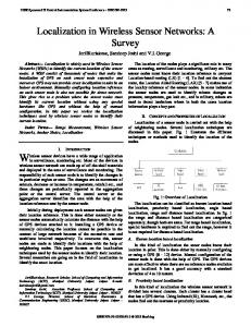
to the life span when it transmits at relatively low power. For this purpose, we have used the MATLAB for the simulation. The simulation result in Fig. 6 and Fig. 9 shows that the activation time of the beacon nodes or the time for which the beacon node is active decrease with the increase in the transmitting power and vice versa. When the beacon nodes transmit at its maximum power then the time for which it is operational will be minimum and the time span will be maximum when it transmit at low power. The simulation results of Fig. 6 and 9 demonstrate the change in time span. Thus these results shows that the power can be conserved and help to increase the longevity of the beacon nodes which is the most important aspect in the process of localization In our proposed model, the beacon node is allowed to transmit at relatively low power then its actual transmitting capacity as it is the only node that has the information in advance regarding its location after the nodes have been deployed. Thus it is important that these beacon nodes remain functional for a longer period of time. Once the beacon nodes transmit, the neighboring node receives the information that has been transmitted by the beacon nodes that consists the identity of the beacon nodes, location and the path length that is set to zero. Now, the distance calculation is done using the free path loss model: D=(c/4*pi*f)(Pt/Pr)1/2 Once the value of the distance is known the next step will be to find the location of the ordinary sensor nodes. For this

After calculation we get, (au, bu ) = (5.3, 2.1) This represents the location of unknown sensor nodes. Thus we are capable of finding the location of the sensor nodes using our proposed algorithm or method. V.

SIMULATION RESULTS AND EXPERIMENTAL VERIFICATIONS

In our proposed model, we have tried to come up with a power efficient method for the localization of sensor nodes. We have also tried to show the inverse relationship between the power transmitted by the Beacon nodes and the life span of the beacon nodes. We have proposed that when the beacon nodes transmit the information at maximum or at high power the life span of the beacon nodes will be shorter as compared

Fig 6

showing the relation between the life span and the power

Fig.7 Calculation of location

purpose we use following method. We find the location of the sensor nodes with respect to the position of the beacon nodes. The calculation of location is represented in Fig. 7. Here we use three beacon nodes to find the location of unknown nodes. Using the distance formula between the beacon nodes and unknown nodes we find the location of the sensor nodes. In the following example we find the location of the unknown nodes with reference to three beacon nodes. Suppose, -

(ai, bi) : coordinates of beacon point i, ri distance to anchor i (a.. b..) : unknown coordinates of node

Using distance formula: - (ai – au )2 + (bi – bu)2 = ri2 for i=1,….,3 - Subtracting eq. 3 from 1 and 2, we get, - (a1 – au )2 – (a3- au)2 + (b1-bu)2 – (b3-bu)2 = (x1)2 – (x3)2 - (a2 - au)2 – (a3- au)2 + (b2 – bu)2 – (b3- bu )2 = (x2)2 – (x3)2 Thus we get the linear equation after rearranging as below:

Arranging the above equation in a matrix form, we get,

This corresponds to AX=B. Using the MATLAB, we can solve the linear equation and get the corresponding value of X as X=A/B

Fig 9. Power is inversely proportional to time span

For Example: Let, (a1, b1)= (3,1), (a2, b2)= (6,5) , (a3, b3)= (9,2), x1=1, x2=2, x3=3

Then,

After calculation we get, (au, bu) = (5.3, 2.1) This represents the location of unknown sensor nodes. The same scenario is illustrated in Fig.8. Thus we are capable of not only finding the location of the sensor nodes but also successfully conserve the power at the same time to increase the longevity of the WSN using our proposed algorithm or method. The simulation result shows that the activation time vary inversely with the transmission power of the beacon nodes and with proper control of the power of the beacon nodes, we can find the location of the sensor nodes in a power efficient manner. VI. CONCLUSION In this paper, we present an algorithm that locates the location of the sensor nodes in a wireless sensor network in a power efficient manner. The simulation results show that the proposed model helps to improve the longevity of the WSN as the method helps to conserve the power which is the main problem in WSN as the sensor nodes have limited power resource and also shows that this method is a power efficient algorithm (i.e., it helps to conserve the power of the node and at the same time find the location of the sensor nodes in Wireless Sensor Network). In future we can make the localization process simpler by using sensors that will not have a battery as it power source i.e., we can use sensors without batteries. REFERENCES [1] [2] [3] [4]

[5] Fig.8. Plotting of the location of the beacon nodes and the unknown sensor nodes after calculating the location of the unknown nodes.

B. Krishnamachari, Networking Wireless Sensors, Cambridge University Press, New York, NY, 2005 S. Rappaport, Wireless Communications, Second Edition, Prentice Hall 2005. B. Nath, D. Niculescu, “Ad-hoc positioning system,” Proc. IEEE Global Communications Conf. (GLOBECOM'01), pp. 2926—2931, 2001. L. Doherty, K. Pister, and L. El Ghaoui, "Convex position estimation in wireless sensor networks," in Proc. 20th Annual Joint Conf. of the IEEE Computer and Communications Society (INFOCOM 2001), Vol. 3, Piscataway, NJ: IEEE Press, 2001, pp. 1655-1663. P. Bergamo and G. Mazzini. Localization in Sensor Networks with Fading and Mobility. In Personal, Indoor and Mobile Radio Communications, pages 750--754, 2002.

[6] [7]

[8]

[9]

[10]

[11]

[12]

[13]

J. Hill, System Architecture for Wireless Sensor Networks. PhD thesis, UC Berkeley, May 2003 X. Ji, H. Zha, Sensor positioning in wireless ad-hoc sensor networks using multidimensional scaling, in: Proceedings of the IEEE INFOCOM, the Annual Joint Conference of the IEEE Computer and Communications Societies, March 2004 G. Balogh, M. Maroti, A. Ledeczi and J. Sallai, “Acoustic ranging in resource constrained sensor network” Technical Report, ISIS-04-504, February 25, 2004 (available at http://www.isis.vanderbilt.edu/publications.asp) W. Su, I. Akyildiz, E. Cayirci, Y. Sankarasubramaniam, “A survey on sensor network" IEEE Communications. Magazine, Vol.40, No.4, pp. 102-114, 2002 Y. Min, K. Won, K. Mechitov, S. Sundresh, W. Kim, G. Agha, “Resilient Localization for Sensor Networks in Outdoor Environment” Distributed Computing Systems, 2005. ICDCS 2005, Proceedings. 25th IEEE International Conference on 10-10 June 2005, pp. 643 – 652 L. Doherty, K. Pister, and L. Ghaoui, “Convex position estimation in wireless sensor networks”. In Proceedings of the 20th Conference of the IEEE Communications Society (IEEE INFOCOM), pages 1655–1663, 2001. D. Niculescu and B. Nath, “Ad-hoc positioning system using AoA”. In Proceedings of the IEEE/INFOCOM 2003, San Francisco, CA, April 2003. Y. Shang and W. Ruml, “Improved MDS-based localization,” Proceedings of the 23rd Conference of the IEEE Communications Society (Infocom 2004); 2004 March 7-11; Hong Kong. Piscataway NJ: IEEE; 2004; 4: 2640-2651

range parallel/distributed systems and the web based training applications. Syed Rizvi is the author of 45 scholarly publications in various areas. His current research focuses on the design, implementation and comparisons of algorithms in the areas of multiuser communications, multipath signals detection, multi-access interference estimation, computational complexity and combinatorial optimization of multiuser receivers, peer-to-peer networking, and reconfigurable coprocessor and FPGA based architectures. AASIA RIASAT is an Associate Professor of Computer Science at Collage of Business Management (CBM) since May 2006. She received an M.S.C. in Computer Science from the University of Sindh, and an M.S in Computer Science from Old Dominion University in 2005. For last one year, she is working as one of the active members of the wireless and mobile communications (WMC) lab research group of University of Bridgeport, Bridgeport CT. In WMC research group, she is mainly responsible for simulation design for all the research work. Aasia Riasat is the author or coauthor of several scholarly publications in various areas. Her research interests include modeling and simulation, web-based visualization, virtual reality, data compression, and algorithms optimization.

Authors Biographies SYED S. RIZVI is a Ph.D. student of Computer Engineering at University of Bridgeport. He received a B.S. in Computer Engineering from Sir Syed University of Engineering and Technology and an M.S. in Computer Engineering from Old Dominion University in 2001 and 2005 respectively. In the past, he has done research on bioinformatics projects where he investigated the use of Linux based cluster search engines for finding the desired proteins in input and outputs sequences from multiple databases. For last one year, his research focused primarily on the modeling and simulation of wide

ALLON RAI is a MS student at University of Bridgeport. He received his B.E degree From Cosmos College of Management and Technology in 2006 and currently enrolled at University of Bridgeport, CT, USA in Electrical department. In the past he has done project in satellite communication. Right now his research area is focused on the Self-Localization of the Wireless Sensor Network, the Wireless Sensor Networks and the power management in the WSN.