A Taxonomy of Localization Schemes for Wireless Sensor Networks

A Taxonomy of Localization Schemes for Wireless Sensor Networks A. Youssef Google Inc. Mountain View, CA, USA

Abstract Knowledge of nodes’ locations is an essential requirement for many applications. This paper surveys the current state of the art for localization schemes in sensor networks. We present a taxonomy of the localization schemes for sensor networks based on different features. We then describe how the current localization schemes for sensor networks map to these different features. We believe that this paper serves as an introduction for researchers interested in the area of localization schemes for sensor networks as well as in evaluating the characteristics of a location system needed by a particular application or the suitability of an existing location system for the application.

Keywords: node localization, scalability, ad-hoc networks, wireless sensor networks, algorithms.

1 Introduction Location discovery in sensor networks have been an active research area for the past couple of years. Applications for localization schemes for sensor networks include determining the location of an event, locationbased routing, e.g. [1], node identification, and node coverage, e.g. [2]. Several localization algorithms have been proposed and implemented. In this paper, we describe a taxonomy that classify the localization schemes for sensor networks based on several distinct features. The taxonomy can be used to understand the key features that distinguish different localization schemes and help in selecting the appropriate scheme for a particular application. In addition it introduces new comers to the area of localization schemes for sensor networks. Based on this taxonomy, we present an overview of the current research in this field of localization schemes for sensor networks by surveying several localization algorithms. This survey helps in understanding the different features of the taxonomy as well as understanding the current state of research in this field.

M. Youssef Computer Science Department University of Maryland College Park, MD, USA The rest of the paper is organized as follows. In Section 2 we present our taxonomy of the localization schemes for sensor networks. Section 3 surveys the current work in the filed of localization schemes for sensor networks. We conclude the paper in Section 4 and give directions for current trends in the area of localization schemes for sensor networks.

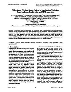
2 Taxonomy Features Location discovery algorithms may be classified according to several criteria, reflecting fundamental design and implementation choices. Those different criteria form a reasonable taxonomy for characterizing and evaluating location discovery algorithms. In this section, we summarize different design alternatives for location discovery algorithms in general and in wireless sensor networks in particular. Figure 1 shows our proposed taxonomy. The rest of this section describes the taxonomy in more details.

2.1

Anchor-based versus Anchor-free

Anchor-based algorithms operate on an ad-hoc network of sensor nodes where a small percentage of the nodes (anchors) are aware of their positions either through manual configuration or using GPS. Anchor nodes broadcast their locations information to their neighbors. The goal is to estimate the positions of as many unknown nodes as possible using anchor node information. Anchor-based algorithms usually produce an absolute location system where absolute node position is known, for example, latitude, longitude, and altitude. However, the accuracy of the estimated position is highly affected by the number of anchor nodes and their distribution in the sensor field [3]. Langendoen et al. [4] showed that with anchor density of 20%, we could have an accuracy of 25% of transmission range, which falls short from the required inaccuracy in many

Localization Schemes for Sensor Networks

Anchor-based

Range estimation

Communication power

Range combining

Computation power

Computational model

Scalability

Accuracy

Capital cost

Figure 1: A taxonomy of localization schemes for sensor networks. applications. Moreover, most of these algorithms suffer from scalability problem. Propagating anchor node location information through the network may lead to a network-wide flooding. Anchor-free algorithms do not make any assumptions regarding node positions. In this case, instead of computing absolute node positions, the algorithm estimates relative positioning, in which the coordinate system is established by a reference group of nodes. In some cases knowing the relative positions of the nodes compared to each other is enough, for example, locationaided routing [5]. Moreover, a relative coordinate system can be transformed to an absolute coordinate system if the coordinates of three separate non-colinear nodes are known in case of 2D (or four in case of 3D). Anchor-free schemes have the disadvantage that when the reference node moves, positions have to be recomputed for nodes that have not moved. This is considered a minor problem in sensor networks where sensor nodes are usually assumed to be stationary.

2.2

Range Estimation Method

Ranging is the process of estimating node-to-node distances or angles. The recent research work by He et al. [6] divides the location discovery algorithms in sensor networks into two major categories: range-based algorithms and range-free algorithms. The former is defined by protocols that use absolute point-to-point range (distance or angle) estimates for estimating location. The later make no assumption about the availability or validity of such information. The most popular methods for estimating the range between two nodes are: • Time-based methods. Time-of-Arrival (ToA) or Time-Difference-of-Arrival (TDoA) methods

record the signal transmission time and the signal arrival time or the difference of arrival times. The propagation time can be directly translated into distance, based on the known signal propagation speed. These methods can be applied to many different signals, such as RF, acoustic, infrared and ultrasound. • Angle-of-Arrival methods. Angle-of-arrival (AoA) methods estimate the angle at which signals are received and use simple geometric relationships to calculate bearings to neighboring nodes with respect to node’s own axis. • Received-Signal-Strength-Indicator (RSSI) methods. Received-Signal-Strength-Indicator (RSSI) methods measure the power of the signal at the receiver. Based on the known transmission power, the effective propagation loss can be calculated. Theoretical and empirical models are used to translate this loss into a distance estimate. This method has been used mainly with RF signals. • Network Connectivity methods. Network connectivity methods can be used for range estimation if the cost of range-estimation hardware is expensive or if a sensor cannot receive signals from enough base stations (≥ 2 for AoA, ≥ 3 for ToA, TDoA, and RSSI). In this case, network connectivity can be exploited for range estimation. For example, the number of hops between two nodes can be used as an estimate of the range between these two nodes.

2.3

Range Combining Technique

Once a location discovery algorithm estimates ranges to other neighboring nodes, it tries to estimate node posi-

B B

C

B

S

A S

A

S

North

D

A

C

(a)

(b)

E

(c)

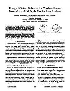
Figure 2: Range Combining Techniques: (a) Trilateration, (b) Triangulation, (c) Multilateration tion using the estimated ranges. The most known techniques for combining ranges are: • Trilateration. Trilateration locates a node by calculating the intersection of three circles as shown in Figure 2a. If the ranges contain error, the intersection of the three circles may not be a single point. • Triangulation. Triangulation is used when the angle of the node instead of the distance is estimated, as in AoA methods. The node positions are calculated in this case by using the trigonometry laws of sines and cosines. In this case, at least two ranges are required as shown in Figure 2b. • Multilateration. In multilateration, the position is estimated from distances to three or more known nodes by minimizing the error between estimated position and actual position. For example, in Figure 2c, we can use the following function to compute the location (x, y) of node S. min

X i

where DS,i

=

p

∧

(DS,i − D )2 ,

(1)

S,i

2.4

Computational Model

There are different possibilities how to construct the localization algorithm and how to divide the computation between nodes. A location discovery algorithm can be categorized under one of the following computational models: • Centralized. In the centralized model, all the range measurements are collected to a central base station where the computation takes place and the results are forwarded back to the nodes. • Locally Centralized. Locally centralized (localized) algorithms are distributed algorithms that achieve a global goal by communicating with nodes in some neighborhood only. For example, the sensor network can be divided into local clusters, where each cluster has a head. All the range measurements in a certain cluster are forwarded to the cluster head where computation takes place. • Fully Distributed. In the fully distributed, computation takes place at every node. In other words, the cluster size is one. Each node is responsible for estimating its own position.

∧

(x − xi )2 + (y − yi )2 , D

S,i

is the estimated range from S to i, i A, B, C, D, E.

=

• Proximity-based. Proximity-based is usually used when no range information is available. In a simple proximity based approach, position of a node is taken as the centroid of positions of connected anchor nodes. An anchor node is considered connected to a node if the percentage of messages received from the anchor node in a time interval t exceeds a certain threshold.

2.5

Accuracy

A location discovery algorithm should estimate sensor position accurately. Accuracy is usually measured as percentage of sensor transmission range. Accuracy usually depends on range measurement errors. Range measurements with less error will lead to more accurate position estimates. Moreover, in anchor-based algorithms, accuracy is affected by the percentage and placement of anchor nodes in the network as well as the placement error.

2.6

Communication Power

Wireless sensors are usually equipped with a limited power source. Therefore energy conservation is one of the major system design factors. A sensor node spends maximum energy in data communication. This involves both data transmission and reception. The current generation of sensor platforms uses about 2 µJ per bit of data transmitted [7]. Usually sensor nodes communicate over a shared medium, and a high density of nodes, coupled with a high messaging complexity, leads to a high collision rate and ultimately to lower throughput and higher power consumption. Therefore, a location discovery algorithm should minimize the amount of node-to-node communication. Data aggregation techniques can be used to conserve communication bandwidth.

2.7

Computation Power

The processor is the second main source of draining battery life. Current small batteries provide about 100mAh of capacity, this can power a small Amtel processor for 3.5 hours (if no power management techniques would be applied) [7]. Energy expenditure in data processing is much less compared to data communication. The example described in [8], effectively illustrates this disparity. Assuming Rayleigh fading and fourth power distance loss, the energy cost of transmitting 1 KB a distance of 100 m is approximately the same as that for executing 3 million instructions by a 100 million instructions per second (MIPS) processor. Hence, a location discovery algorithm should use local data processing in order to minimize communication power.

2.8

Scalability

Scalability is one of the main factors that should be taken into consideration when designing a protocol or an algorithm for sensor networks. The number of sensor nodes in the network may be on the order of hundreds or thousands. Depending on the application, the number may reach an extreme value of millions [7]. For example, a location discovery algorithm should not use flooding to exchange information with other nodes. The sheer number of sensor nodes makes such a global flooding undesirable. A cluster-based approach would work better. Moreover, location discovery systems should not require large tables, which do not fit in the sensor node limited memory.

2.9

Capital Cost

Capital costs include factors such as the price per sensor node or extra hardware required for location determina-

tion. For example, a simple civilian GPS receiver costs around $100. This increases the cost of the sensor node significantly making it impractical to develop.

3 A Survey of Location Discovery Algorithms Node localization has been the topic of active research and many systems have made their appearance in the past few years. In this section we consider several recent localization algorithms for sensor networks. We focus more on the ad-hoc localization problem investigated in the context of sensor networks 1 . The localization algorithm overviews below are intended to emphasize key design issues and how they relate to the taxonomy described in Section 2. Table 1 summarizes the surveyed schemes according to the characteristics described in the Section 2.

3.1

APS Algorithm

The APS algorithm [10] belongs to the class of anchorbased range-free algorithms. Anchor nodes (beacons) flood their location to all nodes in the network using some propagation method. When anchors become aware of other anchor node locations, they use this information to estimate the average hop length in their vicinity and broadcast it back into the network. Nodes with unknown locations also note the shortest hop distance to each of the anchor nodes and multiply it with the broadcasted average hop length to get an approximate distance to each of the anchor nodes. With this information nodes perform a multilateration to get an initial estimate of their locations. The paper discussed three methods of hop-to-hop distance propagation: 1. DV-Hop Propagation Method. Each unknown node records the position and minimum number of hops to at least three beacons. Whenever a beacon, bi , infers the position of other beacons, it computes the average hop distance using Eq.(Eq:APShopDist), and floods this average hop distance √ into the network. Average hop distance =

P

(xi −xj )2 +(yi −yj )2 P ,i hj

6= j

Where hj is the number of hops between beacon bi and bj . Each unknown node then uses the average hop distance to convert hop counts to distances, and performs a triangulation to three or more distant beacons to estimate its own position. 1 For a survey on infra-structure based localization systems, please refer to [9]

APS GPS-less Convex Position Iterative Multilateration GPS-free MDS-MAP Improved MDS-MAP

Anchor

Range Est.

Range Comb.

anchorbased anchorbased anchorbased anchorbased

connectivity trilateration

anchorfree anchorfree anchorfree

Taxonomy Features Comp. Accuracy Comm. Model Power distributed low high

Comp. Power low

Scalability Capital Cost No high

connectivity proximitydistributed based connectivity multilateration centralized

low

low

low

Yes

low

medium

high

high

No

high

ToA

multilateration distributed

high

medium medium No

high

Any

triangulation

medium

high

low

No

low

connectivity multilateration centralized

low

high

high

No

medium

Any

high

low

high

Yes

medium

distributed

multilateration locally centralized

Table 1: Applying the taxonomy to contemporary localization algorithms 2. DV-Distance Propagation Method. This method is similar with the previous one except that distance between neighboring nodes is measured using radio signal strength and is propagated in meters rather than in hops.

3. Euclidean Propagation Method. In this method, the true Euclidean distance to the beacon is propagated. An unknown node needs to know an estimate of distance to at least two neighbors, which have estimates for the distance to a beacon. Then using simple geometry, the unknown node can estimate its distance to the beacon node.

3.2

GPS-less

The GPS-less [11] system is a distributed range-free anchor-based technique. It uses connectivity between nodes in order to estimate node positions. The system employs a grid of beacon nodes , powerful (compared to the nodes) base stations, with known locations; each unknown node sets its position to the centroid of the beacon locations it is connected to. Besides relying on infrastructure support, the accuracy of estimated position depends highly on the density of the beacons. The reported position accuracy is about one-third of the separation distance between beacons.

3.3

Convex Position Estimation

Convex position algorithm [12] belongs to the class of centralized range-free anchor-based localization algorithms. The algorithm uses the connectivity between nodes to formulate a set of geometric constraints and solve it using convex optimization. If one node can communicate with another, a proximity constraint exists between them. For example, if particular RF system can transmit 20m and two nodes are in communication, their separation must be less than 20m. These constraints restrict the feasible set of unknown node positions. Formally, the network is a graph with n nodes at the vertices and with bidirectional communication constraints as the edges. Positions of the first m nodes, anchor nodes, are known (x1 , y1 ...xm , ym , ) and the remaining n − m positions are unknown. The problem is then to find (xm+1 , ym+1 ...xn , yn ) such that the proximity constraints are satisfied. The algorithm is based on semi-definite programming and requires rigorous computation so it is not always suitable for sensor networks. The resulting accuracy depends on the fraction of anchor nodes. A serious drawback is that convex optimization is performed by a single, centralized node; hence; it is not suitable for many ad-hoc setups.

3.4

Iterative Multilateration

Iterative multilateration [13] is used in the AHLoS project. The algorithm is fully distributed and can run on each individual node in the network. An unknown

node u that is connected to at least three beacons can estimate their position by solving the following system of equations: d2iu = (xi − xu )2 + (yi − yu )2 ∀u ∈ U and i ∈ Bu (2) Where Bu is the set of all beacon neighbors of u. The resulting system of equations can be linearized by rearranging terms, and subtracting the last equation from the rest to obtain the following equation: ai xu +bi yu = ci , where ai , bi , andci are constants. (3) This system of equations can be solved using the matrix solution for minimum mean square estimate (MMSE) [13]. Once a node estimates its position it becomes a beacon and can assist other unknown nodes in estimating their positions by propagating its own location estimate through the network. This process iterates to estimate the locations of as many nodes as possible. Iterative multilateration requires high fraction of beacon nodes. It is sensitive to beacon densities and can easily get stuck in places where beacon densities are sparse. Another drawback of iterative multilateration is the error accumulation that results from the use of unknown nodes that estimate their positions as beacons.

3.5

GPS-free

In their GPS-free system [14], Capkun et al introduced the Self-Positioning Algorithm (SPA) that enables nodes in a MANET to find their positions in the network using range measurements between the nodes. The TOA method is used to obtain range between two mobile devices. Each node in the network builds its own local coordinate system by assuming itself as the origin of this coordinate system, and selecting two noncollinear one-hob neighbors to form axes. Then the positions of one-hop neighbors are computed accordingly. The local coordinate systems at each node can have different directions so another phase is required to map all the local coordinate systems of the nodes to the network coordinate system. This is done through simple matrix rotations and may be mirroring. To compute the network coordinate system, a subset of nodes is chosen (Location Reference Group) such that it is stable and less likely to disappear from the network. Then the network coordinate center is chosen to be the geometrical center of the location reference group and the direction of the network coordinate system is the mean value of all directions of the local coordinate systems of the nodes belonging to location reference group. As the nodes move, the location reference group is periodically updated using expensive message broadcast. Moreover,

the network center and direction are recomputed using expensive message broadcast. The work was focusing on the network mobility and how this affects the localization accuracy. Power consumption at each node was not considered as a major problem.

3.6

MDS-MAP

MDS-MAP [15] is a localization method based on multidimensional scaling (MDS). It determines the positions of nodes given only basic information that is likely to be already available, namely, which nodes are within communications range of which others. If the distances between neighboring nodes can be measured, that information can be easily incorporated into the method. MDS-MAP is able to generate relative maps that represent the relative positions of nodes when there are no ”anchor” nodes that have known absolute coordinates. When the positions of a sufficient number of anchor nodes are known, e.g., 3 anchors for 2-D localization and 4 anchors for 3-D, MDS-MAP then determines the absolute coordinates of all nodes in the network. MDSMAP often outperforms previous methods when nodes are positioned relatively uniformly in space, especially when the number of anchors is low. MDS-MAP uses the distance or connectivity information between all nodes at the same time, whereas previous triangulationbased methods localize one unknown node at a time and only use the information between the unknown and anchor nodes. However, like many existing methods, MDS-MAP does not work well on irregularly-shaped networks, where the shortest path distance between two nodes does not correlate well with their true Euclidean distance.

3.7

Improved MDS-MAP

In [16], an enhanced version of MDS-MAP is proposed that works well on both uniform and irregular networks. The main idea is to compute a local map using MDS for each node consisting only of nearby nodes, and then to merge these local-area maps together to form a global map. The new technique is called MDS-MAP(P), which stands for MDS-MAP using patches of relative maps. This approach avoids using shortest path distances between far away nodes, and the smaller local maps, constructed using local information, are usually quite good. An optional refinement step using least-square minimization may be used to refine the relative maps computed by MDS. MDS is often good at finding the right general layout of the network, but not the precise locations of nodes. That makes the MDS solution a good starting point for the local optimization done in the re-

finement step. The refinement improves solution quality but is much more expensive than MDS. MDS computes analytical solutions in O(n3 ), where n is the number of nodes. Thus, the refinement provides a trade-off between solution quality and computational cost.

[7]

[8]

4 Conclusions and Trends This paper presented a taxonomy of the different features that can be used to classify localization schemes for sensor networks and a survey of the current localization schemes for sensor networks. The paper serves as an introduction to new comers to the field of localization schemes for sensor networks. Moreover, in addition to simply reasoning about a location-sensing system, our taxonomy can be applied to evaluate the characteristics of a location system needed by a particular application or the suitability of an existing location system for the application. Current trends of the field of localization schemes for sensor networks include scalable localization schemes, localization using new transmission technologies, e.g. ultra wideband and WiMax, and localization for new classes of sensor network, e.g. building structure sensor networks.

References [1] B. Karp and H.T. Kung. Greedy perimeter stateless routing for wireless networks. In International Conference on Mobile Computing and Networking, pages 243–254, Boston, MA, 2000. [2] Seapahn Meguerdichian, Farinaz Koushanfar, Miodrag Potkonjak, and Mani B. Srivastava. Coverage problems in wireless ad-hoc sensor networks. In INFOCOM, pages 1380–1387, 2001. [3] Nirupama Bulusu, J. Heidemann, V. Bychkovskiy, and D. Estrin. Density-adaptive beacon placement algorithms for localization in ad hoc wireless networks. In IEEE Infocom 2002, June 2002. [4] K. Langendoen and N. Reijers. Distributed Localization in Wireless Sensor Networks: A Quantitative Comparison. Computer Networks (Elsevier), special issue on Wireless Sensor Networks, pages 374–387, August 2003. [5] I. Stojmenovic and X. Lin. Loop-free Hybrid Single-path Flooding Routing Algorithms with Guaranteed Delivery for Wireless Networks. IEEE Transactions on Parallel and Distributed Systems, 12(10):1023–1032, October 2001. [6] T. He et al. Range-free localization schemes for large scale sensor networks. In the Proceedings of

[9]

[10]

[11]

[12]

[13]

[14]

[15]

[16]

the ACM Conference on Mobile Computing and Networks (MOBICOM’03), September 2003. I.F. Akyildiz, W. Su, Y. Sankarasubramaniam, and E.Cayirci. Wireless sensor networks: a survey. Computer Networks, 38(4):393–422, 2002. G. J. Pottie and W. J. Kaiser. Wireless integrated network sensors. Communications of the ACM, 43(5):51–58, April 2000. Jeffrey Hightower and Gaetano Borriella. Location Systems for Ubiquitous Computing. IEEE Computer, 34(8):57–66, August 2001. D. Niculescu and B. Nath. Ad-hoc positioning system. In the Proceedings of IEEE Global Communication Conference (Globcom’01), November 2001. N. Bulusu, J. Heidemann, and D. Estrin. GPSless Low-cost Outdoor Localization for Very Small Devices. IEEE Personal Communications, 7(5):28–34, October 2000. L. Doherty, K. Pister, and L. El Ghaoui. Convex position estimation in wireless sensor networks. In the Proceedings of IEEE Conference on Computer Communications (INFOCOM), April 2001. A. Savvides, C. C. Han, and M. Srivastava. Dynamic fine-grained localization in ad-hoc networks of sensors. In the Proceedings of the ACM Conference on Mobile Computing and Networks (MOBICOM’01), July 2001. S. Capkun, M. Hamdi, and J.-P. Hubaux. Gpsfree positioning in mobile adhoc networks. In Hawaii International Conference on System Sciences (HICSS-34), pages 3481–3490, January 2001. Yi Shang, Wheeler Ruml, Ying Zhang, and Markus P. J. Fromherz. Localization From Mere Connectivity. In the Proceedings of ACM MOBIHOC 2003, pages 201–212, Annapolis, MD, June 2003. Y. Shang and W. Ruml. Improved mds-based localization. In the Proceedings of IEEE Conference on Computer Communications (INFOCOM), March 2004.