Department of Computer Science & Engineering,. Indian Institute of ... republish, to post on servers or to redistribute to lists, requires prior specific permission ...
A New Performance Evaluation Approach for System Level Design Space Exploration C.P. Joshi, Anshul Kumar and M.Balakrishnan Department of Computer Science & Engineering, Indian Institute of Technology Delhi, India {cpjoshi,mbala,anshul}@cse.iitd.ernet.in
ABSTRACT Application specific systems have potential for customization of design with a view to achieve a better costperformance-power trade-off. Such customization requires extensive design space exploration. In this paper, we introduce a performance evaluation methodology for system-level design exploration that is much faster than traditional cycleaccurate simulation. The trade off is between accuracy and simulation speed. The methodology is based on probabilistic modeling of system components customized with application behavior. Performance numbers are generated by simulating these models. We have implemented our models using SystemC and validated these for uni-processor as well as multiprocessor systems against various benchmarks.
Categories and Subject Descriptors C.3 [Special-purpose and Application-based Systems]: Real-time and embedded systems; C.4 [Performance of Systems]: Modeling techniques, measurement techniques
General Terms Performance, Design, Experimentation
Keywords Design space exploration, statistical simulation, system level design
1.
INTRODUCTION
A system designer is faced with a large number of architectural choices while designing a system for a specific application. To obtain the best solution, a designer needs to evaluate performance for various design alternatives. Performance evaluation approaches can be broadly categorized as analytical and simulation based. Analytical approaches aim at closed form solutions which lead to quick evaluation of performance [6, 7, 8, 1, 4]. However, they
Permission to make digital or hard copies of all or part of this work for personal or classroom use is granted without fee provided that copies are not made or distributed for profit or commercial advantage and that copies bear this notice and the full citation on the first page. To copy otherwise, to republish, to post on servers or to redistribute to lists, requires prior specific permission and/or a fee. ISSS’02, October 2–4, 2002, Kyoto, Japan. Copyright 2002 ACM 1-58113-576-9/02/0010 ...$5.00.
have limitations in one way or other. For example, some approaches are limited in terms of their ability to take into account application characteristics (e.g. [6]) or interaction among multiple processors (e.g. [8, 1]) or instruction level details of the processors (e.g. [6, 7, 8, 4]. Because of such limitations of analytical models, cycle accurate simulation is the most commonly used approach for performance evaluation of system. The drawbacks of cycle accurate simulation is that it is very time consuming. Each design point requires complete simulation of the architecture with application mapped on to it. For real applications, each simulation run can be quite long. Keeping in mind these drawbacks of existing techniques, we have developed a new methodology which adopts a middle path between analytical and cycle-accurate simulation. We use probabilistic models for components, customized with application behavior. We have adopted simulation of probabilistic models because averaged performance numbers converge very fast. The models are at a higher level of abstraction which results in faster simulation, at the expense of slightly reduced accuracy. The methodology can handle multiprocessor systems containing processors and applicationspecific hardware. The models are generic and can handle a variety of components. This methodology can be useful in the following scenario: 1. Evaluating system performance at higher level for narrowing down design alternatives. 2. Evaluating communication cost for a given application running on processor or application-specific hardware, in a multiprocessor environment. 3. Studying effects of read/write buffers with in a single processing element for a given application. Another approach which adopts a middle path between analytical and simulation is reported by Mark Oskin [9]. However, his work is limited to a small range of architectures and for uni-processors only. Statistical models are simplistic and cannot account for the read/write buffer performance. In the next section we describe the basic idea behind our approach. In Section 3 we discuss the overall methodology. In Section 4, we define the modeling of various architectural features and customization of models based on application behavior. In Section 5, we have described validation and experimental results of our modeling and simulation technique. Finally conclusion and future work is discussed in Section 6.
lw Address
r1 PC
Instruction
r2
1000
1 Request 1
Update 7
2
Ack
IR
Processor
2
Reg File
Memory
3
Memory Data
6
RegFetch Processor
Address
5
3
Request 5
Address Calculation 4
Ack
(a) Conventional Cycle-accurate Simulation
7
4 Delay
6
(b) Our Simulation
Figure 1:
2.
BASIC IDEA
To discuss the basic idea behind our approach, we consider an example of a non-pipelined processor without buffers and cache. To execute a load word instruction lw, r1, 1000(r2), the operation sequence performed by a conventional cycle accurate simulator will be as shown in Figure 1(a). Our simulator aims at reproducing only the event timings, ignoring actual data transfers and computations. The timings of the reproduced events are required to match the actual timings in statistical sense only. Thus, our simulator generates only request and acknowledge events when the cycle accurate simulator performs instruction fetch and data fetch, as shown in Figure 1(b). Other steps of cycle accurate simulation such as register fetch, address calculation, PC update etc. are simply replaced by delays in our approach. In this example, the delays between the events are fixed, but in general, these may be generated randomly with some probabilistic distribution. Performance metrics are calculated from various statistics gathered during the course of simulation by monitoring state of simulator at appropriate points in models. Example of some metrics are: a) Component utilization, b) Memory and interconnection bandwidths, c) Fraction of interconnection bandwidth used by various components, d) Processor CPI, e) Stalls due to Read/Write and Prefetch Buffer, f) Pipeline stalls etc.
3.
tural feature level, b) Partitioning level, wherein only the component-task binding is changed and c) System level, which involves varying number and types of components as well as the partitioning. This may be done interactively or using scripts. Target System Architecture and Component Features
Application
HW/SW Partitioning and Binding
Modify Architecture
Modify Partitioning
A Target Arch. Simulator Generator
Parameter Extractor
Architectural Component Simulation Model Library
Binding Info Only
Target Arch. Simulator
Application Parameters
Simulator Customization
THE METHODOLOGY
The overall methodology for performance evaluation in the context of system-level design exploration is shown in dotted box A in Figure 2. This is part of the larger Automated Synthesis of Embedded Systems, ASSET project [3]. The methodology takes as input the partitioned application, target system architecture containing component architectures and interconnections, and the binding information of application partitions to architectural components. The methodology can be divided in to five parts: Model Library building, application parameter extraction, target architecture simulator generation, customization of simulator and simulation and performance number generation. Models library building is a one time process and is discussed in Section 4, other parts are discussed here. The dotted lines in Figure 2 indicate that the design space exploration may be carried out at a) Component architec-
Cycle by Cycle Simulation
Performance Numbers
Figure 2: Design Flow for Performance Evaluation
3.1 Application Parameter Extraction Application behavior is represented in the form of statistical parameters. These parameters are explained in detail in section 4. These parameters can be generated by either a) Static analysis and profiling of the application along with
cache simulation if needed or b) From some existing simulation framework, like SimpleScalar [2]. We wish to make it clear that the parameters of applications are independent of architecture, hence, parameters extraction is a one time process.
Instr. Class
Architectural Parameters Number of words to be loaded
Load Store
Number of words to be stored
Control
-
Compute (others)
Cycles for execution stage(EX)
3.2 Simulator Generation Target system architecture is input to this step. In this step simulator is generated for target system by instantiating specified components from model library and connecting them through ports according to given interconnection specifications. Component models are built using SystemC. The generated simulator can be visualized as shown in figure 3. Each model has two major parts : its functionality and statistical data gathering and some housekeeping functions. Functionality
Application Parameters Distributions of load instructions or the size of clustered load Distributions of store instructions or the size of clustered store branch instruction distribution, prob. of branch taken Distributions of instructions and the number of EX cycles
Table 1: Processor instruction classification with their architectural and application parameters
Instances of library components
4.1 Processor Model 11111 00000 00000 11111 00000 11111 00000 11111 00000 11111 00000 11111 00000 11111 00000 11111 00000 11111 00000 11111 00000 11111 00000 11111 00000 11111 00000 11111 00000 11111 00000 11111 00000 11111 00000 11111 00000 11111 00000 0000011111 11111 0000011111 0000011111 0000011111 00000 11111 SystemC Library Houskeeping/Statistics gethering
Figure 3: Software Aspects of Simulator Generation Model library contains generic definition of components like processor, specialized hardware, memory, buffers etc. Their feature parameters are decided according to given input specification. It makes the methodology generic at subcomponent and their feature level. Components can be conveniently interconnected through abstract ports.
3.3 Simulator Customization This is the stage where captured behavior of the application in terms of statistical parameters is used to customize the respective component of generated system simulator, as specified by binding information. For each partition of the application the following binding information is required: a) Processing element to which it is bound b) Memory where program is stored and c) Memories where data are stored. In this customization, the respective processing element’s probabilistic event generation process is tuned using application parameters. Here event generation refers to selection of next state of processing element from probability distribution, for example instruction and memory access data size. Hereafter we will refer to the probabilistic distribution as distribution.
4.
MODEL LIBRARY
A key part of our methodology is model library containing probabilistic models of components. These models are created by focusing only on terminal behavior and delays. Major system level components that we have considered are processors, application-specific hardware, buses, memories, caches and write/read buffers. Application parameters considered for modeling are specific to a component and its features. In the following subsections we describe a few of these models.
For processor modeling we presently consider only RISC type processors in our framework. However, it is possible to incorporate CISC type processors with minor modifications. We next describe in detail the various factors considered while modeling a processor. We consider architectural features and parameters like cycle time, word size, pipelining, size of instructions, number of ports and their size, program and data memory ports, instruction prefetch buffer size, on-chip cache and its parameters, write and read buffers. In figure 4 an abstract architectural model of a processor is shown with five stage instruction pipeline, instruction prefetch, write and read buffer. Dotted arrows show the request and ack and solid arrows show flow of information of transaction like amount of data to be transferred. As we are interested only in terminal behavior and delays, we have classified instruction in four generic classes. Table 1 shows the instruction classification along with their selected application and architectural parameters used to define a processor model. Distribution of size of clustered load and store is helpful in capturing the bursty nature of application for memory access. We describe in detail modeling of write and read buffers in Sections 4.5 and 4.6.
00 11 00 11 00 11 00 11 00 11 00 11
0 000 111 1111 000 0 1 1111 0000 0 1 111 000 0 1111 000 0 1 111 000 1111 0000 0 1111 000 0 1
Inst. prefetch Buffer
D
AG DF/DS EX WB
Read Buffer
Write Buffer
Req/Ack
Port Interface
Bus
Inst. Pipeline
Processor A
Target Architecture Processor B ASIC C Memory
Transaction Info
Figure 4: Abstract Architectural Model of A Processor For modeling instruction pipeline, generic instruction execution templates are defined for each class of instructions which can be parameterized for the specific architecture. A cycle increment model is adopted. In this model we assume the ideal pipeline performance to be one CPI. Effect of hazards like stalls, pipeline flush etc. are counted by simply inserting a number of additional penalty cycles.
4.2 Application Specific Hardware Model
4.4 Bus Model
There is no notion of memory access for instruction fetch in application specific hardware. However memory communication is required for accessing data before and after processing. In case the data itself is large then memory accesses are required even during processing. The performance of an application depends on the available FUs, pipelined and non-pipelined implementation, data access time from memory etc. Hardware implementation determines the rate of external data access. Performance of application specific hardware considering fixed penalty for data access can be evaluated by simply scheduling operations considering available FUs. However to determine overall performance we have to add data access time which itself is a function of effective memory bandwidth. In our hardware model we use a hardware estimator[3], which gives estimated execution time of application on hardware excluding external data access. Table 2 shows considered application parameters for application specific hardware.
Considered features are cycle time, data width, burst/nonburst transfers, arbitration type, components connected. Even though we have only validated bus based systems, the framework is not specifically meant for buses only and one can plug any type of interconnection model.
PaDisDisDis-
Write Distance Distribution
Description Obtained from hardware estimator. Frequency of various data sizes for reads (in words). Frequency of various data sizes for write (in words). Frequency of distances between two successive reads (in number of cycles). Frequency of distances between two successive writes (in number of cycles).
Write buffers are subcomponents used to improve processor performance. Memory write stalls are reduced by using write buffers. Just considering Store Instruction Distribution is not sufficient for performance evaluation of processors with write buffers, because performance of write buffers depends upon the time interval of store instructions. To capture this behavior we compute either the store instruction distance distribution or build a Markov model. Store Instruction Distance Distribution is the dynamic instruction distance between store instructions. During simulation, next buffer distance is determined from this distribution on occurrence of a write to the buffer. The above model can be improved by modeling distances between stores using Markov Chains in terms of basic operations. At any occurrence of store, next distance is determined from the distance distribution for the current distance. This is explained by the following example: for (i = 0; i < 50; i + +) do for (j = 0; i < 100; j + +) do A[i] = i*j; end for end for
Table 2: Application Parameters for H/W
Features for memory that have been considered include cycle time, word size, access latency, degree of inter-leaving and number of ports. Delay models have been used for memory. Using delay model the total memory busy time is calculated. One of the delay models used to calculate the time for which memory remains busy is given below:
99
1
Distance 5
1 Distance 9
49
Figure 5: Markov model ords−1)+M emLatency ⌉ M CR = ⌈ BusCycleT ime×(ReqBusW M emoryCycleT ime
Where MCR is required memory cycles and ReqBusWords is the number of bus words requested for memory access.
4.3.1 Cache Model Features of cache considered are type of cache (I-cache, D-cache and unified cache), capacity, line size, access time and write policy. Application parameters extracted are hitratio and dirty line probability. We obtain this information from Dinero IV cache simulator [5]. Defining mean miss distance (mmd) in number of hits, we generate next cache (nm) miss randomly, assuming exponential inter miss distance using a uniform random number generator in the interval zero and one (U[0, 1]). mmd =
hit ratio and nm = −mmd ∗ log (U [0, 1]) 1 − hit ratio
mov mul store incr compare jump incr compare jump Basic operations of example code Distance outer loop = 9
4.3 Memory Model
Distance inner loop = 5
Application rameter Execution Time Read Data Size tribution Write Data Size tribution Read Distance tribution
4.5 Write Buffer Model
Store Distance
A Markov model is shown in figure 5, where a state represent a distance of stores. Index variables are stored in registers and arrays are stored in memory and accessed through load and store instructions. In this case, the distance between two array assignment is 5 and in each iteration of outer loop this distance occurs 99 times. 100th time it goes to outer loop and that makes a distance of 9.
4.6 Read Buffer Model Read buffers are data prefetch buffers which are used in systems where the reading of data are predictable in application. Media applications are examples of such applications. For example, consider convolution computation where a mask is moved on an image frame. Processing time for each move is fixed and the pixels to be processed in the next move are known. In such cases, data read requests can be put much earlier than their actual need. It improves the data read delays in systems.
Parameters 32-bit 10 ns 3 stage Unified 8KB, WTNWA 4 addresses, 8 words 40 ns, 32-bit,no inter-leaving 40 ns, 32-bit
Table 3: ARM710a based uni-processor system specifications To model read buffer, we need information about read requests sent to the read buffer, as well as the points where data is actually read from buffer during execution. Relevant application parameters that we have used are Data Read Request Size Distribution, Data Read Request Distance Distribution and Buffer Read Distance Distribution, which is the distribution of distances between consecutive buffer reads for which requests have been already placed. As explained in the write buffer models, Markov models may also be used.
5.
VALIDATION
In order to validate our models and simulation methodology with existing architectures and simulators, we use ARM710a and Cradle UMS [10] as uni-processor and multiprocessor architectures respectively. The ARM simulator, ARMulator was running on an HP PA-RISC platform with HP-UX and the UMS architecture simulator was running on Pentium class workstation with MS Windows. The experimental setups and results are explained as follows.
5.1 Uni-Processor System We have used ARM710a processor with a bus and a memory. Specifications of our interest are given in table 3. Experiments have been done for various benchmarks mentioned in table 4. The biquad N section program, part of DSPkernel benchmark suite [11], performs filtering of input values through N biquad IIR sections. lattice init calculates the output of a lattice filter, me ivlin is a media application, mainly consisting of integer arithmetics, whereas matrix mult implements multiplication of 2D matrices. Results have been validated against the ARMulator, a functional simulator for ARM processor family and provides cycle-counts. We have compared the performance numbers that can be extracted from ARMulator simulation information and are shown in table 4. In the last column, if the values of metric are absolute then percentage error has been considered. On the other hand if values of metric are already in percentage then only the absolute difference has been considered. Host times shown in Our Simulation columns are the convergence times. It is clear from comparison that the simulation results are within 10% of ARMulator results and convergence time is much less then the time taken by ARMulator. Convergence time is independent of size-of application, where size is in terms of code and execution time, but depends upon the variance in various distributions.
5.2 Muli-Processor System Validation for multiprocessor systems has been done for Cradle Technologies UMS (Universal Micro System) [10]. The UMS is a single chip stream-processing architecture, consisting of clusters of processors connected by a 64-bit
Performance Metric lattice init CPI Bus Util.(%) Bus Bandw.(MB/sec) Processor Util.(%) Host Time(sec) biquad N sections CPI Bus Util.(%) Bus Bandw.(MB/sec) Processor Util.(%) Host Time(sec) me ivlin CPI Bus Util.(%) Bus Bandw.(MB/sec) Processor Util.(%) Host Time(sec) matrix mult CPI Bus Util.(%) Bus Bandw.(MB/sec) Processor Util.(%) Host Time(sec)
ARMulator
Our Simulator
Diff. Abs./%
4.5237 65.2032 21.7344 74.9857 5.37
4.34092 70.6239 23.5468 64.3639 1.9
4.04 % -5.42 8.33 % 10.62
2.5143 73.877 24.6259 72.082 9.69
2.598 74.3893 24.797 67.135 2.0
-3.32 % -0.51 -0.69 % 4.94
1.2855 4.14 1.3466 98.91 17.07
1.30945 3.64982 1.2166 97.2309 2.1
-1.86 % 0.490 9.65 % 1.67
2.11386 50.06422 16.6880 92.8949 17.53
2.08219 48.3603 16.1200 95.887 2.3
1.49 % 1.70 3.40 % -2.99
Table 4: Comparison between ARMulator and our simulation results for ARM710a based uni-processor system high bandwidth global bus. These processor clusters, called Quads, communicate with external DRAM and I/O interfaces. A Quad of the UMS is shown in Figure 6. Each Quad consists of 4 RISC-like non-pipelined processors called PEs, 8 DSP-like processors called DSEs, a local 16KB data memory, a local 12KB instruction memory/cache, a memory transfer engine, a local 64-bit data bus and 64-bit instruction bus. Each DSE has a read and write buffer.
PE 3
MTE
Features Word Size Cycle Time Pipelined Cache Write Buffers Memory Bus Cycle Time
PE 2
PE 1
PE 0
Global Bus Interface
Instruction Bus Data Bus
Instruction Cache/ Memory Data Cache/ Memory
DSE DSE DSE DSE DSE DSE DSE DSE 7 6 5 4 3 2 1 0 Figure 6: A Quad of UMS architecture Modeling of DSE has been done as application specific hardware because it has large number of registers and its own local instruction memory. A 720x480 colored image filter application has been used as benchmark. Two quads i.e. 8 PEs and 16 DSEs are used for filtering. Image is divided in 16 independent groups each having 30 consecutive rows and each DSE processes one group of rows. A copy of filter program is mapped to each
63 "ums_filter−2_PE_Utilization" 62
% Utilization
61
extended for system-level power estimations. Presently we have modeled only RISC type processors, more efforts are needed to model architectures like VLIW, superscalar and multithreaded processors.
60 59
7. ACKNOWLEDGMENTS
58
This methodology is developed as a part of ASSET project at Indian Institute of Technology Delhi.
57 56
8. REFERENCES
55
[1] A. Allara, Carlo Brandolese, William Fornaciari, Fabio Salice, and Donatella Sciuto. System-Level Performance Estimation Strategy for SW and HW. In Proc. ICCD, October 1998. [2] Douglas C. Burger and Todd M. Austin. The SimpleScalar Tool Set, Version 2.0. Technical Report CS-TR-1997-1342, 1997. [3] ASSET: Automated Synthesis of Embedded Systems, IIT Delhi. http://www.cse.iitd.ernet.in/esproject. [4] A. Van Gemund. Performance Modeling of Parallel Systems. PhD thesis, Delft University of Technology, Apr. 1996. [5] EM. Hill. Dinero-IV Manual. NEC Research Institute, 1997. [6] Lizy Kurian John and Yu cheng Liu. Performance Model for a Prioritized Multiple-Bus Multiprocessor System. IEEE Transactions on Computers, 45(5):580–588, 1996. [7] D. R. Liang and S. K. Tripathi. On Performance Prediction of Parallel Computations with Precedent Constraints. IEEE Transactions on Parallel and Distributed Systems, 11(5):491–508, 2000. [8] Derek B. Noonburg and John Paul Shen. A Framework for Statistical Modeling of Superscalar Processor Performance. In 3rd International Symposium on High Performance Computer Architecture, San Antonio, TX, pages 298–309. [9] Mark Oskin, Frederic T. Chong, and Matthew Farrens. HLS: Combining Statistical and Symbolic Simulation to Guide Microprocessor Designs. In Proc. International Symposium on Computer Architecture (ISCA00), 2000. [10] http://www.cradle.com/ums/architecture.html. [11] V. Zivojnovic, J. Velarde, and C. Schlager. Meyr: DSPStone – A DSP-oriented Benchmarking Methodology. In Int. Conf. on Signal Processing Applications and Technology(ICSPAT), 1994.
54
0
100000
200000
300000
400000
500000
600000
Processor Cycle * 100
Figure 7: Simulation Convergence DSE, whereas PEs are only used to initialize and control DSEs. Table 5 shows the comparison of various performance numbers interpreted from SSi (Soft Silicon), a UMS architecture simulator and simulation performed by our simulator. As the same application is mapped to all similar DSEs and same function is performed by all used PE, results for all PEs, and DSEs are identical. Again here we have compared only the metrics that are can be either extracted or available by SSi results. Performance Metric PE CPI DSE Utilization(%) Local Data Bus packets/cycle(%) Global Bus packets/cycle(%) Host Time (sec) 1 frame
SSi Simulator 5.80161 21.262
Our Simulator 5.950668 23.974
Diff. Abs./% -0.02569 % -2.712
38.329
35.606
2.723
11.698
8.717
2.981
1380
14
Table 5: Comparison of performance numbers of our simulation with UMS’s SSi simulator Host times shown in Our Simulation column is the convergence time. It is clear from comparison that the simulation results are again within 10% of SSi simulator results and convergence time is much less then the time taken by SSi simulator. Figure 7 shows the convergence of PE utilization. SSi simulation takes 66285280 UMS cycles for one frame processing, but our simulation converges within 2% much before 100000 cycles of simulation.
6.
CONCLUSION AND FUTURE WORK
We have presented a probabilistic model based simulation methodology for performance evaluation. This is a faster technique as compared to cycle-accurate simulation, it can be used in early system design phase to narrow down the design alternatives. Even though simulation converges very fast, it depends upon the variance of application parameter distributions. We need to develop a technique to preprocess this distribution to ensure a fast convergence. According to our experience with this research, the models can be