transfer functions and takes into account a polariser presence or absence. Using the ..... free spectral range of FSR=2100GHz, and a 2nd order Butter- worth electrical ..... [7] B. Saleh, M. Teich, âFundamentals of photonicsâ, John. Wiley & Sons ...
NEW GAUSSIAN APPROXIMATION FOR PERFORMANCE EVALUATION OF OPTICAL RECEIVERS WITH ARBITRARY OPTICAL AND ELECTRICAL FILTERS João L. Rebola and Adolfo V. T. Cartaxo Abstract A new Gaussian approximation (GA) which takes into account the influence of arbitrary optical and electrical filters is proposed for the performance evaluation of optically preamplified receivers. Using the new GA, the receiver sensitivity is evaluated and notable performance differences were observed for several Fabry-Perot optical filters. I. INTRODUCTION The Gaussian approximation (GA) has been utilised to evaluate the performance of optically preamplified receivers. Its inherent simplicity, relative accuracy, and short computation time have been sufficient reasons to use it. Several GA have been proposed [1-6], however none of them can fully accommodate the influence of arbitrary optical and electrical filters. In [1], rectangular optical and electrical filters have been assumed, as well as constant signal power, and a simplified AG has been derived considering an approximated signal-dependent noise variance calculated over the total average signal. In [2,3] a rectangular optical filter with much larger bandwidth than the bit rate has been considered, and the GA presented allows to take arbitrary electrical filters into account. In [4], a GA for a large bandwidth optical filter and a short-term integrator as electrical filter has been presented. In [5,6], a Lorentzian shape for the optical Fabry-Perot (FP) filter has been assumed, and the mean and variance depend on eigenvalues obtained from Karhunen-Loève signal and noise expansions, and do not present explicitly the dependence on the electrical and optical filter transfer functions. In this work, a new GA that accommodates arbitrary optical and electrical filters is presented. Furthermore, this GA also takes into account the effects of waveform distortion in the signal and in the signal-spontaneous emission (ASE) beat noise. Exact expressions for the mean and variance of the current at the decision circuit input are derived, which clearly present the dependence on the optical and electrical filters transfer functions and takes into account a polariser presence or absence. Using the GA, the receiver sensitivity is evaluated for different kinds of FP optical filters and electrical filters. J. Rebola and A. Cartaxo are with the Optical Communications Group, Dept. Electrical and Computers Engineering, Instituto de Telecomunicações, Instituto Superior Técnico, Pólo I, 1049-001 Lisboa, Portugal. This work was supported by FCT and POSI within project POSI/35576/CPS/2000 - DWDM/ODC. J. Rebola would like to thank FCT for supporting this work also under contract SFRH/BD/843/2000.
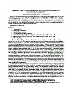
II. OPTICALLY PREAMPLIFIED RECEIVER MODEL The block diagram of the optical receiver is shown in Fig. 1. The optical receiver includes a preamplifier with flat gain ! G, which amplifies the received electrical field ein (t ) , and ! adds ASE noise e ASE (t ) to the signal. ! e ASE (t )
! e in (t )
! ! ! ! esA (t ) + enA (t ) e s (t ) + e n (t )
Polariser
G Optical preamplifier
H o (f) Optical filter
PIN
Sampling
i(t) Decision circuit
H r(f) Electrical filter
id (t)
Fig. 1 Block diagram of optical receiver.
The signal and noise fields are assumed to have arbitrary polarisations. An arbitrary polarisation can be expanded as a weighted superposition of two orthogonal Jones vectors [7]. Hence, the signal and noise fields are given, respectively, by
! ! ! ein (t ) = ein, x (t )⋅ x + ein , y (t )⋅ y
(1)
! ! ! e ASE (t ) = e ASE , x (t )⋅ x + e ASE , y (t )⋅ y
(2)
where ein,x(t), eASE,x(t) and ein,y(t), eASE,y(t) are the received signal and the ASE noise components over the orthogonal ! ! directions defined by the unit vectors, x and y , respectively. Usually, the signal field is considered with one polarisation state [1-6], and in this situation, the two noise orthogonal polarisation modes are referred to as parallel (to the signal) and orthogonal modes. With no loss of generality, if we consider the signal is linearly polarised in one direction, ! ! either x and y , the assumption of one signal polarisation state is accomplished. The ASE noise is assumed as optical additive white Gaussian noise (AWGN) with power spectral density in each orthogonal direction given by SASE=nsp(G-1)hν with nsp the spontaneous emission noise factor and hν the photon energy. The polariser transmits the electrical field component in the ! ! x direction and blocks the orthogonal component in the y direction. The effect of the polariser can be described by ! ! ! (3) e sA (t ) = G ein, x (t )⋅ x + G ( p − 1) ⋅ ein , y (t )⋅ y
! ! ! e nA (t ) = e ASE , x (t )⋅ x + ( p − 1) ⋅ e ASE , y (t )⋅ y
(4)
where we set p=1 or p=2, respectively, in the presence or absence of a polariser.
The signal is then filtered by an optical filter with impulse response and transfer function expressed, respectively, as ho(t) and Ho(f), and with a -3dB bandwidth, Bo. We assume that the optical filter acts equally over the two directions. The ! ! output filtered signal is e s (t ) + e n (t ) , with ! ! (5) e s (t ) = e sA (t ) ∗ ho (t ) ! ! (6) e n (t ) = e nA (t ) ∗ ho (t ) where * stands for the convolution operation. ! The complex envelopes of the ASE noise, n ASE (t ) , and of ! the received field, s in (t ) , are defined, respectively by [2]
{ ! 2 Re{s
! ! e ASE (t ) = 2 Re n ASE (t )⋅ e j 2πν ot ! ein (t ) =
in
(t )⋅ e
j 2πν o t
}
}
(7)
{
H o ( f ) = H o ,l ( f − ν o ) +
}
H o*,l (−
f −ν o )
(8)
(9) (10)
For the lowpass-equivalent model, from expressions (1), (2), (5) and (6), we have ! ! ! (11) s A (t ) = G s in, x (t )⋅ x + G ( p − 1)⋅ s in , y (t )⋅ y
! ! ! n A (t ) = n ASE , x (t )⋅ x + ( p − 1)⋅ n ASE , y (t )⋅ y
(12)
! ! s (t ) = s A (t )∗ ho ,l (t )
(13)
! ! n (t ) = n A (t )∗ ho,l (t )
(14)
! ! ! where s (t ) and n (t ) are the complex envelopes of e s (t ) and ! e n (t ) , respectively. The PIN photodetector is assumed as a square-law detector with responsivity Rs, and the PIN output current i(t) is [8]
! ! 2 i(t ) = R s s (t ) + n (t )
(15)
The subsequent electrical circuitry is modelled by an electrical filter with impulse response and transfer function, respectively, hr(t) and Hr(f), and a -3dB bandwidth, Be. Its output current id(t), which is given by i d (t ) = i (t )∗ h r (t )
−∞
[
{[ G s
in, x
(τ1 ) + nASE, x (τ1 )]⋅ [
][
(16)
is sampled and a decision circuit decides on the transmitted symbols. To estimate the receiver performance through the GA, it is necessary to derive expressions for the mean and variance of id(t). From (11)-(16), id(t) can be expressed as
]
* * G sin , x (τ 2 ) + nASE, x (τ 2 ) +
]}
* * + ( p − 1)⋅ G sin, y (τ1 ) + nASE, y (τ1 ) ⋅ G sin , y (τ 2 ) + n ASE, y (τ 2 ) ⋅
⋅ ho,l (χ − τ1 )⋅ ho*,l (χ − τ 2 )⋅ hr (t − χ ) dτ1dτ 2 dχ
(17) III. GAUSSIAN APPROXIMATION From (17), the mean and variance deduction is straightforward, but lengthy. Details can be found in Appendix A. Exact expressions for the mean and variance of id(t) which explicitly present the dependence on the transfer functions of the arbitrary filters are, respectively, +∞
where νo is the optical carrier frequency. The lowpass equivalent of the impulse response, ho,l(t), and transfer function, Ho,l(f), of the optical filter are defined by ho (t ) = 2 Re ho ,l (t )⋅ e j 2πν ot
+∞
id (t ) = Rs ∫ ∫∫
+∞
2 2 µ (t ) = pRs S ASEH r (0) ∫ Ho,l ( f ) df + RsG ∫ sin, x (τ )∗ ho,l (τ ) + −∞ −∞ (18) 2 + ( p − 1)⋅ sin, y (τ )∗ ho,l (τ ) ⋅ hr (t − τ ) dτ
[
+∞
]
2 σ 2 (t ) = 2 Rs2GS ASE ∫ { sin, x (τ ) ∗ ho,l (τ ) ⋅ hr (t − τ )}∗ ho,l (τ ) + −∞
+ ( p − 1) ⋅
{[sin, y (τ )∗ ho,l (τ )]⋅ hr (t − τ )}∗ ho,l (τ ) 2 dτ +
(19)
+∞
2 2 2 2 + pRs2 S ASE ⋅ ∫ H r ( f ) H o,l ( f ) ∗ H o,l ( f ) df −∞
The first term of (18) is the mean current component due to the spontaneous emission noise and the second one is the signal component. In (19), the first term is the signal-ASE beat noise and the second term is the ASE-ASE beat noise. The receiver performance is estimated analytically through the error probability. Using a GA, the error probability is given by [6] 1 N −1 F − µ 0, k Pe = ⋅ ∑ Q σ 0,k N k =0 (ak = 0 )
N −1 µ1, k − F + ∑ Q (20) k =0 (a =1) σ 1, k k
where N is the total length of the binary sequence; ak is the kth symbol, either ‘0’ or ‘1’; F is the threshold level; Q(x) is defined in [2]; and µi,k and σi,k are, respectively, the mean and standard deviation of id(t) conditioned by the symbol i and at the sampling instant, tk=k/B+to, with k=0,...,N-1, where to can be chosen in order to optimise the system performance and B is the bit rate. The optimal threshold level, Fopt, is obtained from N −1
∑
1
σ 0, k k =0 (ak =0 )
1 Fopt − µ 0, k exp − 2 σ 0, k
1 1 µ1, k − Fopt exp − = ∑ 2 σ 1, k k = 0 σ 1, k (ak =1) N −1
2
=
2
(21)
which results from setting to zero the derivative of (20) with respect to F.
IV. COMPARISON WITH OTHER AUTHORS’ RESULTS
V. NUMERICAL RESULTS
Through appropriate simplification, and considering that ! the signal is polarised in the x direction and p=1, expressions (18) and (19) degenerate in the mean and variance expressions presented in [1-5]. In this section, these simplifications are explained for the cases considered in Ref. [1] and [2,3].
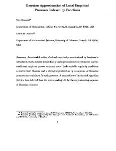
In this section, the receiver sensitivity estimated by the new GA is compared with the one obtained with the GA presented in [2,3] and their features are discussed. Then, the new GA is used to estimate the receiver performance for several optical and electrical filters. ! With no loss of generality, the signal is polarised in the x direction. The parameters considered for the receiver are G=30dB, nsp=2, B=40Gbit/s, Rs=1A/W, N=64, p=1, rectangular pulse shapes are assumed for the binary sequence. The sensitivity is calculated for the error probability of 10-12. In Fig. 2, the sensitivities obtained with the new GA and the GA in [2,3] are depicted. A single-cavity FP filter [9] with free spectral range of FSR=2100GHz, and a 2nd order Butterworth electrical filter with Be=0.65B are considered. In order to compute the receiver sensitivity using the GA presented in [2,3], a rectangular optical filter with the same equivalent noise bandwidth (within the FSR) as the FP filter is assumed, and the optical signal is filtered by the FP optical filter.
A. Rectangular optical filter In Ref. [2,3], a large bandwidth rectangular optical filter is assumed with lowpass equivalent transfer function H o ,l ( f ) = rect ( f Bo )
(22)
where rect(f) stands for the rectangular function with unit width. It is also assumed that the optical filter does not affect the received signal. Starting from the relation H o ,l ( f ) ∗ H o ,l ( f ) = B o Λ ( f B o ) 2
(23)
where Λ(f) is the triangular function defined by
-25
1 − f Bo , f < Bo Λ ( f Bo ) = otherwise 0,
(24)
and substituting (22) and (23) in (18) and (19), the mean and variance expressions are given, respectively, by +∞
µ (t ) = R s S ASE Bo H r (0 ) + R s G ∫ P(χ )⋅ hr (t − χ ) dχ
(25)
−∞
[
]
+∞
+∞
2
-27 -29 -31
20
(26)
2 − Rs2 S ASE ∫ f ⋅ H r ( f ) df
GA in [2] and [3]
-33
2 Bo ∫ H r ( f ) df − σ 2 (t ) = 2Rs2 S ASEG P(t )∗ h2r (t ) + Rs2S ASE −∞
New GA
Sensitivity [dBm]
2
2
60 100 140 180 220 260 300 340 B o [GHz]
Fig. 2 Sensitivity vs optical filter bandwidth.
−∞
where the optical power at the receiver input is given by P(t)=|sin(t)|2. Since Bo is assumed considerably larger than the bit rate, the third term of (26) can be neglected and, thus, the mean and variance expressions coincide with the expressions presented in [2,3].
B. Rectangular electrical filter and constant signal power In addition to the rectangular optical filter, in Ref. [1] the signal is considered as having constant power, sin(t)= P , and the electrical filter is a rectangular filter with bandwidth Be and unit gain. It is also assumed that the optical filter acts only over the ASE noise and does not affect the input signal. In this case, expressions (25) and (26) simplify to
µ (t ) = R s S ASE Bo + R s GP
(27)
(
2 2 Bo Be − Be2 σ 2 (t ) = 4 R s2 S ASE GPBe + R s2 S ASE
)
(28)
which correspond to the mean and variance expressions presented in [1].
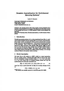
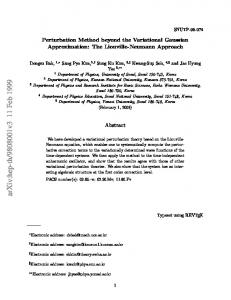
From Fig. 2, discrepancies between the results estimated by the two GA are obvious. Sensitivity differences of 5dB are found for lower Bo. For larger Bo, the mean and the variance achieved by the GA presented in [2,3] tend to (18) and (19), as shown in section IV.A. The new GA can also plainly estimate an optimal bandwidth for the optical filter, whereas the GA presented in [2,3] does not give this information so clearly. In Fig. 3 and 4, the new GA is used to estimate the receiver performance with three different optical filters: the singlecavity FP filter, the double-cavity FP filter [9] and the threemirror FP filter [10]. In Fig. 3 and Fig. 4, the electrical filter is a 2nd and a 6th order Butterworth with Be=0.65B, respectively. Fig. 3 and 4 show that the three-mirror FP filter leads to worse sensitivity behaviour. The sensitivity behaviour for the single- and double-cavity FP filter is very alike, but the double-cavity FP filter performance is slightly worse than the single-cavity FP filter performance.
Sensitivity [dBm]
-25 single-cavity FP double-cavity FP three-mirror FP
-27 -29 -31 -33 20
40
60
80 100 120 B o [GHz]
140
160
single-cavity FP filter with Bo=40GHz and for the 2nd and 6th order Butterworth filters. Fig. 5 shows that the optimal electrical filter bandwidth is about 30GHz and 32GHz, for the 2nd and the 6th order Butterworth filters, respectively. The bandwidth of the electrical filter used in Fig. 3 and 4 was Be=24GHz (0.65B). For this electrical filter bandwidth, as shown in Fig. 5, the 6th order Butterworth filter leads to a sensitivity degradation above 1dB, whereas the 2nd order Butterworth leads to less than 0.5dB degradation, in comparison with the optimum electrical filter bandwidths observed in Fig. 5. This explains the worst performance of the 6th order Butterworth filter observed in Fig. 4.
Fig. 3 Sensitivity vs optical filter bandwidth for the 2nd order Butterworth filter.
single-cavity FP double-cavity FP three-mirror FP
-27 -28
Butt2
Sensitivity [dBm]
Sensitivity [dBm]
-26
-28 Butt6
-29 -30 -31
-29 -32
-30
16
24
32
-31 20
40
60
80 100 120 B o [GHz]
140
160
64
72
80
Fig. 5 Sensitivity vs electrical filter bandwidth for the singlecavity FP filter.
Fig. 4 Sensitivity vs optical filter bandwidth for the 6th order Butterworth filter.
-28 24GHz
Sensitivity [dBm]
For lower optical bandwidths, the intersymbol interference (ISI) effect dominates the sensitivity degradation. So, filters with sharper cut-off and higher delay slope in the passband edge (as the three-mirror FP) lead to worse receiver performance, because they introduce higher ISI. With the increase of the optical filter bandwidth, the influence of the ASE noise increases and the ISI introduced by the optical filter decreases. There is a point where the two impairments lead to the maximum sensitivity. That maximum corresponds to the optimal optical filter bandwidth. For the three-mirror FP filter this optimal bandwidth corresponds to 50GHz and 35GHz, with the 2nd and 6th order Butterworth electrical filter, respectively. For the single- and double-cavity FP filter, this bandwidth is about 55GHz and 37 GHz, with the 2nd and 6th order Butterworth electrical filter, respectively. Beyond this optimal bandwidth the sensitivity degradation is mainly due to the signal-ASE beat noise. The choice of the electrical filter is also important. From Fig. 3 and 4, the receiver performance is worst for the electrical filter with sharper cut-off and higher delay slope (6th order Butterworth filter). The performance differences can be above 1dB for the optimal and larger optical bandwidths. The sensitivity behaviour observed in Fig. 4 is not as smooth as the one observed in Fig. 3. This is due to the electrical filter bandwidth choice. In Fig. 5, the optimisation of the electrical filter -3dB bandwidth is estimated for a
40 48 56 B e [GHz]
32GHz
-29 -30 -31 -32 20
40
60
80 100 120 B o [GHz]
140
160
Fig. 6 Sensitivity vs optical filter bandwidth for the 6th order Butterworth filter with different -3dB bandwidths.
Fig. 6 shows that with the optimised electrical filter bandwidth, the receiver sensitivity turns out to be much better than with Be=24GHz for the 6th order Butterworth filter, for the optimal optical filter bandwidth and above. VI. CONCLUSIONS The new GA is a fast and simple method to analyse the receiver performance for arbitrary optical and electrical filters, and this arbitrariness is a great advantage above other GA [1-7]. It allows the estimation of the optimal optical and electrical filters bandwidth, and hence it is an important tool in the design of optically preamplified receivers with tight optical filtering, such as the typical of high dense-wavelength division multiplexing systems.
Future work should investigate the accuracy of the sensitivities estimated through the new GA by comparison with estimates obtained using more rigorous methods.
The assumption of the ASE noise as AWGN leads to the properties
⋅ δ (τ 1 − τ 2 )]⋅ ho,l (χ 1 − τ 1 )⋅ ho*,l (χ 1 − τ 2 )⋅ ho*,l (χ 2 − τ 3 )⋅
E [n A (t )] = 0
(29)
⋅ ho,l (χ 2 − τ 4 )⋅ hr (t − χ 1 )⋅ hr (t − χ 2 ) dτ 1 dτ 2 dτ 3 dτ 4 dχ 1 dχ 2 (34)
E nA (t1 )⋅ n*A (t2 ) = S ASEδ (t1 − t2 )
(30)
By subtracting (33) by (34), the variance can be written as
[
]
(31) E[nA (t1 )⋅ nA (t2 )] = 0 ! ! where nA(t) stands either for x or y directions. Other important properties are: the odd order moments of gaussian processes with zero average are null, and orthogonal components are uncorrelated. Using (17), (29), (30) and (31), the mean is given by
[
+∞
E [i d (t )] = µ (t ) = R s ∫ ∫∫ Gs in , x (τ 1 )⋅ s in∗ , x (τ 2 ) + G ( p − 1)⋅ −∞
( ) (τ 2 ) + pS ASE δ (τ 1 − τ 2 )]⋅ h o ,l (χ − τ 1 )⋅ ⋅ h o*, l (χ − τ 2 )⋅ h r (t − χ ) d τ 1 d τ 2 d χ
∗ ⋅ s in , y τ 1 ⋅ s in ,y
(32)
where the relation (p-1)2=(p-1) for p=1 and 2 is used. From now on, the determination of (18) from (32) is simple and involves only the integrals simplification. The autocorrelation term is given by
]
* ⋅ δ (τ 4 − τ 3 ) + pGS ASE s in , x (τ 4 )s in , x (τ 3 )δ (τ 1 − τ 2 ) + 2( p − 1)⋅ * 2 ⋅ GS ASE s in, y (τ 4 )s in , y (τ 3 )δ (τ 1 − τ 2 ) + 2 p ⋅ S ASE δ (τ 4 − τ 3 )⋅
APPENDIX A
[
* * ⋅ s in , x (τ 2 )δ (τ 4 − τ 3 ) + 2G ( p − 1)S ASE s in , y (τ 1 ) s in , y (τ 2 )⋅
+∞
[
* * E id (t ) ⋅ id* (t ) = Rs2 ∫ ∫∫∫∫∫ G2sin, x (τ1 ) sin , x (τ 2 ) sin, x (τ 3 ) sin, x (τ 4 ) +
−∞ * + G2 p − 1 sin, x τ1 sin ,x
( ) ( ) (τ 2 ) sin* , y (τ3 ) sin, y (τ 4 ) + G2 ( p − 1)sin, y (τ1) ⋅ * * 2 * * ⋅ sin , y (τ 2 ) ⋅ sin, x (τ 3 ) ⋅ sin, x (τ 4 ) + G ( p − 1)sin, y (τ1 ) sin, y (τ 2 ) sin, y (τ 3 ) ⋅ * sin, y (τ 4 ) + pGSASEsin, x (τ1 )⋅ sin , x (τ 2 )δ (τ 4 − τ 3 ) + 2G( p − 1)S ASE ⋅ * * ⋅ sin, y (τ1 ) sin, y (τ 2 )δ (τ 4 − τ 3 ) + GSASEsin, x (τ 4 ) sin , x (τ 2 )δ (τ1 − τ 3 ) + * * + G( p − 1)S ASE sin, y (τ 4 ) sin , y (τ 2 )δ (τ1 − τ 3 ) + GSASE sin, x (τ1 ) sin, x (τ 3 ) ⋅ * ⋅ δ (τ 4 − τ 2 ) + G( p − 1)S ASE sin, y (τ1 ) sin , y (τ 3 ) ⋅ δ (τ 4 − τ 2 ) + pGSASE ⋅ * * ⋅ sin, x (τ 4 ) ⋅ sin, x (τ 3 )δ (τ1 − τ 2 ) + 2( p − 1)GSASEsin, y (τ 4 )sin , y (τ 3 ) ⋅ 2 2 ⋅ δ (τ1 − τ 2 ) + 2 pSASEδ (τ 4 − τ 3 )δ (τ1 − τ 2 ) + pSASEδ (τ 4 − τ 2 ) ⋅ ⋅ δ (τ1 − τ 3 )]⋅ ho,l (χ1 − τ1 ) ⋅ ho*,l (χ1 − τ 2 ) ⋅ ho*,l (χ2 − τ 3 ) ⋅ ho,l (χ2 − τ 4 ) ⋅ ⋅ hr (t − χ1 ) ⋅ hr (t − χ2 ) dτ1dτ 2dτ 3dτ 4dχ1dχ2 (33) where the relations (p-1)2=(p-1) and (p-1)4=(p-1) for p=1 and 2 are used. From (17), we obtain
[ ]
+∞
[
* * E [i d (t )]E i d* (t ) = R s2 ∫ ∫∫∫ ∫∫ G 2 s in , x (τ 1 ) s in , x (τ 2 ) s in , x (τ 3 )⋅ −∞
* * s in , x (τ 4 ) + G 2 ( p − 1)s in , x (τ 1 ) s in , x (τ 2 ) s in , y (τ 3 ) s in , y (τ 4 ) + * * + G 2 ( p − 1)s in , y (τ 1 )⋅ s in , y (τ 2 )s in , x (τ 3 )⋅ s in , x (τ 4 ) + ( p − 1)⋅ * * ⋅ G 2 s in , y (τ 1 ) s in , y (τ 2 ) s in , y (τ 3 )s in , y (τ 4 ) + pGS ASE s in , x (τ 1 )⋅
+∞
[
[
σ 2(t ) = Rs2 ∫ ∫∫∫∫∫ GSASE sin, x (τ4 ) sin* , x (τ2 ) + ( p −1)sin, y (τ4 )⋅
]
−∞
[
* * ⋅ sin , y (τ2 ) ⋅ δ (τ1 −τ3 ) + GSASE sin, x (τ1 ) sin, x (τ3 ) + ( p −1)sin, y (τ1 )⋅
]
* 2 sin , y (τ3 ) δ (τ4 −τ 2 ) + pSASEδ (τ4 −τ2 )⋅ δ (τ1 −τ3 )]⋅ ho,l (χ1 −τ1 )⋅ (35)
⋅ ho*,l (χ1 −τ2 )⋅ ho*,l (χ2 −τ3 )⋅ ho,l (χ2 −τ4 )⋅ hr (t − χ1)⋅ hr (t − χ2 )⋅ ⋅ dτ1dτ2dτ3dτ4dχ1dχ2 From expression (35), the variance presented in (19) can be obtained by performing the integrations over τ1, τ2, τ3 and τ4, and then, by simplifying the resulting integrals. VII. REFERENCES [1] N. Olsson, “Lightwave systems with optical amplifiers”, J. Lightwave Tech., pp. 1071-1082, July 1989. [2] L. Ribeiro, J. da Rocha, J. Pinto, “Performance evaluation of EDFA preamplified receivers taking into account intersymbol interference”, J. Lightwave Tech., pp. 225-231, Feb. 1995. [3] S. Danielsen et al., “Detailed noise statistics for an optically preamplified direct detection receiver”, J. Lightwave Tech., pp. 977-981, May 1995. [4] P. Humblet, M. Azizo~ glu , “On the bit error rate of lightwave systems with optical amplifiers”, J. Lightwave Tech., pp. 1576-1582, Nov. 1991. [5] I. Monroy, G. Einarsson, “Bit error evaluation of optically preamplified direct detection receivers with Fabry-Perot optical filters”, J. Lightwave Tech., pp. 1546-1553, Aug. 1997. [6] C. Lawetz and J. Cartledge, “Performance of optically preamplified receivers with Fabry-Perot optical filters”, J. Lightwave Tech., pp. 2467-2474, Nov. 1996. [7] B. Saleh, M. Teich, “Fundamentals of photonics”, John Wiley & Sons, Inc., Ch. 6, 1991. [8] L. Kazovski, S. Benedetto, A. Willner, “Optical fiber communication systems”, Artech House, Ch. 2, 1996. [9] P. Humblet, W. Hamdy, “Crosstalk analysis and filter optimization of single- and double-cavity Fabry-Perot filters”, J. Sel. Areas Comm., pp.1095-1107, Aug. 1990. [10] J. Stone, L. Stulz, A. Saleh, “Three-mirror fibre FabryPerot filters of optimal design”, Electr. Lett., pp. 10731074, July 1990.