International Conference on Power Systems Transients – IPST 2003 in New Orleans, USA
A New Approach for Integration of Two Distinct Types of Numerical Simulator Hongtian Su, L. A. Snider and K. W. Chan, Baorong Zhou Dept. of Electrical Engineering, The Hong Kong Polytechnic University, Hung Hom, Kowloon, Hong Kong SAR, PRC (e-mail:
[email protected],
[email protected],
[email protected])
the advantages of both EMTP and TSP. They achieved this by simultaneously performing TSP and EMTP with periodic coordination of the results. Some further studies have been done since then [3-5]. Whether or not to extend the interface location further has been discussed extensively in these papers, based on the same interface protocol proposed in [2]. This paper describes new developments for the enhanced interface of EMTP and TSP which would be capable of running in real time.
Abstract – Electromagnetic transient simulation and electromechanical transient simulation are two distinct types of simulators, based on different modeling techniques. EMTP comprises a three-phase simulation engine which can accommodate phase unbalance and waveform distortion. TSP produces phasor solutions, usually only positive sequence, in the time domain. This paper presents a hybrid simulator, based on interfacing the two types of simulators. Hybrid simulation has the advantages of being computationally inexpensive while providing detailed dynamic modeling of systems containing nonlinear components such as HVDC and FACTS devices. By exchanging information between EMTP and TSP at specified time intervals, the two simulation engines can be integrated together almost seamlessly. Some of the problems associated with the interface and a new protocol which successfully solves the interface problems are described. A case study of an SVC interfaced to a 9-bus 3machine system, demonstrates the accuracy of the approach.
II. OVERVIEW OF HYBRID SIMULATION Since the hybrid simulation contains two simulation engines, the network is partitioned into two parts, the detailed system (EMTP type simulation) and the external system (TSP type simulation). The integration time step of TSP is usually in the order of several milliseconds, while that for EMTP, when modeling power electronic apparatus at the device level, is in the order of microseconds. The two simulations proceed in parallel and at specified time points they communicate with each other. With the interchange of information each part of the network is represented to the other by an equivalent.
Keywords – electromagnetic transient program, transient stability program, hybrid simulation, Norton equivalent, SVC
I. INTRODUCTION In this paper we are dealing with two basic power simulation tools: the electromagnetic transients program (EMTP) [1] and the transient stability program (TSP), also known as electromechanical transient program. Electromagnetic transient programs solve in the time domain usually with small time steps (in the order of microseconds) and can provide detailed solutions over a very wide bandwidth but for relatively small systems. Transient stability programs are based on fundamental frequency, positive sequence solutions, and use integration time step in the order of milliseconds. TSP takes relatively much less computation time and can simulate very large size network in real-time. The application of power electronics devices in power system, such as FACTS and HVDC, lead to onerous demands on power system simulation techniques: power electronic devices require very small time steps to be properly represented at the device level. This cannot be accommodated in conventional transient stability program, consequently these devices are represented as quasisteady-state models, which only account for the normal working conditions. Valve malfunctions, for example, cannot be adequately represented. In the early eighties, Heffernan et al. first proposed the interface of two distinct simulators to solve HVAC-HVDC systems. They modeled an HVDC link in detail within a stability based ac system framework [2], thus exploiting
TSP calculation step T0 T1
T2
T3
EMTP calculation step
Fig. 1 Interaction Protocol of Hybrid Simulation
The interaction and communication between the detailed system (the EMTP simulation) and the rest of the network (the TSP simulation) is maintained through a well-defined interfacing bus. The factors involved in achieving the proper interaction of the detailed system (EMTP) and external (TSP) systems include [4]: 1. selection of interaction locations, 2. modeling of an equivalent for the external system in the detailed analysis, 3. modeling of an equivalent for the detailed system
1
International Conference on Power Systems Transients – IPST 2003 in New Orleans, USA
in the external system, the protocol for interaction between the external and the detailed systems. In this paper the detailed system refers to an SVC (Static Var Compensator), connected to an external system which is simulated by a TSP program.
d-axis sub-transient parameters are equal to the q-axis subtransient parameters (this is always true in the case of a thermal unit), the equivalent circuit of the generator can be represented as shown in Figure 2.
4.
A. Interaction Location The choice of the interface location depends on the scale of detailed system and the accommodation of nonfundamental components presented by non-linear elements. There are two different approaches to choose the interface location. The obvious approach takes the SVC installation bus as the point of interface location. This minimizes the size of the detailed system, so that the EMTP computation time can be reduced to a minimum. The disadvantage is that when the external network is represented by a simple fundamental frequency equivalent, the equivalent representing the external network system may be too simple, particularly for weak system, since the effect of other frequencies presented by the detailed part will be not taken into account. The alternative is to extend the interface location further into the external network [3], so that the waveforms of interfacing buses will be more sinusoidal. This will also facilitate data transfer from EMTP to TSP. How far should the interface location be extended depends on two factors: phase imbalance and waveform distortion. As the interface location is extended, the number of interfacing buses is generally increased. Another countermeasure to the first approach, which does not need to extend the interface location, is to develop an equivalent that can fully replicate the dynamic behavior of the original external system [4]. When EMTP is running, a fundamental frequency equivalent is substituted by a multi-pole equivalent [6-7]. Thus the harmonics generated by detailed part can be fully considered.
Fig. 2 Equivalent Circuit of a Thermal Generator
The value of equivalent current source is a function of generator state variables and sub-transient parameters and the equivalent internal impedance is jx d" , which can be incorporated into the network to establish the equivalent. If we define that under dq reference the q axis leads d axis by 90 degree and angle d is the angle by which q axis leads the y axis, the relationship between the dq reference and xy reference can be summarized by the following equation. V dq e
π jδ − 2
= V xy
(1)
Then the generator injection current is, Eqi" sin δ i E " cos δ I x + jI y = − di " i + " xdi xqi
" E " sin δ Eqi cos δ i j − di " i − " x x qi di
(2)
The information (sources value) transferred from TSP to EMTP is only three-phase fundamental frequency positive sequence quantities that are converted from phasor values calculated by TSP. In EMTP the external system is represented in terms of these quantities. C. Modeling of Detailed System in TSP There are several different ways to represent an equivalent detailed network, such as an SVC, in the transient stability program. We can roughly separate them into two groups; one is at mathematical level and the other at the device level. Mathematical models presuppose that the device works as designed; malfunctions, such as valve failures, cannot be adequately represented. This limitation does not exist in the device level modeling, where the non-linear elements can be represented at the device level. Generally, the outputs from EMTP can be unbalanced, distorted waveforms. However TSP is based on fundamental frequency positive sequence modeling techniques, consequently the information from EMTP to TSP must be fundamental frequency positive sequence quantities, which may include bus voltages, current, active power and reactive power. In this paper, the variables are fundamental active power and reactive power, which are extracted from distorted waveforms. Thus, the device is viewed by TSP as a load.
B. Modeling of External System in EMTP To the EMTP simulation, the external system needs to be represented by a correct driving point impedance. The TSP is a fundamental frequency phasor-like solution, and at each interchange it can provide fundamental frequency voltage, current and equivalent impedance. This is presented to the EMTP simulation at the interface bus as a Norton equivalent which includes a current source and an RLC network. For a simple Norton equivalent, there is only one series RLC shunt-connected circuit, however this simple equivalent cannot give correct waveforms following changes of topology. A more comprehensive frequency dependent equivalent comprises a number of RLC shuntconnected circuit. Since the external network parameters in TSP are constant, the parameters for RLC circuits are also constant. Therefore, only the source value is updated at every interchange, and this is determined by the generators in TSP. Consider, for example, a sub-transient model of a generator. If the sub-transient model is used in TSP, where the 2
International Conference on Power Systems Transients – IPST 2003 in New Orleans, USA
D. Interaction Protocol
Transfer Norton equivalent to EMTP
In TSP the integration step is in the order of milliseconds while in EMTP it is in the order of microseconds. Because different integration time steps are adopted by the two simulation packages, information exchanging occurs only at some common time points: usually at the TSP time steps. This is illustrated in Figure 1. All the proposed hybrid simulators [3-5] are based on the following implementation of interfacing protocol (refer to Figure 3): t0
t1
5
Run TSP
t1
t0
t2 5
TSP
1
4
2
EMTP
3
Transfer information to TSP
Run EMTP
t2
Fig. 4 Flow Chart for the New Proposed Protocol 1
2 4
IV. INTERACTION ANALYSIS In the hybrid simulation the Norton equivalent current source seen by the EMTP simulation remains constant between successive interchange intervals. Consequently, there is a discontinuity caused by the step change in the current source at the interchanges, as shown in Figure 5.
3
Fig. 3 Interaction Protocol 1
1. 2.
EMTP and TSP run from time t0 to time t1. The Norton equivalents for the external system are obtained from TSP at t1 and are transferred to EMTP. 3. Using the Norton equivalent obtained at t1 from TSP, EMTP is executed from t1 to t2. 4. The accumulated EMTP data from t0 to t2 are processed by using curve fitting in order to obtain phasor values of V, I, P and/or Q and transferred to TSP at t1. 5. TSP is executed from t1 to t2 using the updated information at t1. 6. The above procedure is repeated With this protocol the phasor values are transferred to the TSP at the beginning of the TSP calculation interval. However, transient stability programs require a prediction of the bus voltages and loads at t2 in order to do the calculation for the interval t1 to t2. We can provide this in real time with the following protocol, where both simulators are running faster than real time: 1. EMTP and TSP run sequentially from time t0 to time t1. 2. The Norton equivalents for the external system are obtained from TSP at t1 and are transferred to EMTP. 3. Using the Norton equivalent obtained at t1 from TSP, EMTP is executed from t1 to t2, while the TSP process is idle. 4. The EMTP data from t1 to t2 are processed by using curve fitting in order to obtain phasor values of P and Q corresponding to time t2. 5. TSP uses the P and Q from EMTP to do the calculation for the interval t1 to t2, which include required iterations, while the EMTP processors are idle. 6. The above procedure is repeated.
I n' In
tn
Fig. 5 Step Change of Current Source The effect of this discontinuity is, however, small, as can be seen in Figure 6, where there is an interchange at 2.8 second. From the bus voltage waveform it is obvious that the transient process caused by the step magnitude change can be reasonably ignored. 5
2
x 10
1.5
Bus Voltage (V)
1
0.5
0
-0.5
-1
-1.5
-2 2.78
2.785
2.79
2.795
2.8
2.805
2.81
2.815
2.82
Time (second)
Fig. 6 Interface Bus Voltage The most significant factor which can affect the performance of the hybrid simulation is the system frequency variation which occurs during electromechanical transients. This leads to a phase angle shift in the bus voltage at each TSP interval, as illustrated in Figure 7. Suppose the system frequency is transiently greater than 50 Hz, as shown by the dotted (lower) curve of bus voltage. The solid (top) 3
International Conference on Power Systems Transients – IPST 2003 in New Orleans, USA
curve represents the bus voltage at the EMTP bus, developed by the Norton equivalent running at a fixed frequency of 50Hz. The resulting phase shift leads, effectively, to a discontinuity, which produces a spurious transient which in turn, as shown in Figure 8, causes a significant distortion and unbalance in voltage waveforms.
interval. Rather, the exchange should take place when there is no phase angle error of the interface bus voltage, thus eliminating the discontinuity. The success of this method will be demonstrated with the following case study. 5
6
2.5
x 10
4
2 2
Bus Voltage (V)
1.5 1
0.5
0
0
-2
-0.5 -4
-1
-1.5 -6 -2 -2.5
0
0.5
1
1.5
2
2.5
3
3.5
4
3.5
4
Time (second) 0
0.002
0.004
0.006
0.008
0.01
0.012
0.014
0.016
0.018
0.02
Fig. 10 Unbalanced Interface Bus Voltage
Fig. 7 System Frequency Variation
5
6
x 10
5
2.5
x 10
4
2
1.5 2
Bus Voltage (V)
3-Phase Bus Voltage (V)
1
0.5
0
0
-2
-0.5
-1 -4 -1.5
-2 -2.5 2.78
-6
0
0.5
1
1.5
2
2.5
3
Time (second) 2.785
2.79
2.795
2.8
2.805
2.81
2.815
2.82
Time (second)
Fig. 11 Balance Interface Bus Voltage
Fig. 8 Distortion Caused by Phase Shift
V. CASE STUDY A three-machine-nine-bus system [8], shown in Figure 9, is used as test network. An FC/TCR (Fixed Capacitor/Thyristor Controlled Reactor) type SVC is connected to the bus 9. The three TCR branches are delta-connected, and, for simplicity, the shunt capacitor and TCR are directly connected to the bus, not through a transformer. A 5th harmonic filter is connected to the same bus. Loads are represented by constant impedance models, and the SVC controller is described in [9]. At 0.5 seconds a three-phaseto-ground fault is applied to bus 7, and at 0.8 second the fault is successfully cleared. We have two sub-systems: the network part and the SVC. For the network part the transient stability program is employed with a 20 milliseconds integration step. EMTP is used to simulate SVC with a 50 microseconds integration step. The SVC installation bus is chosen as interfacing bus.
Fig. 9 Benchmark System Schematic Diagram This problem related to waveform distortion and unbalancing has not been reported previously. The solution to this problem lies in not restricting the exchange of data between the two simulations at a fixed
4
International Conference on Power Systems Transients – IPST 2003 in New Orleans, USA
The external system is represented by a simple Norton equivalent in EMTP. The SVC is viewed by TSP as a load, that is, SVC is represented by a fundamental component of P and Q, which can be extracted from distorted waveforms. This case study is mainly focused on the effect of detailed modeling of the SVC on the predicted stability of the system. The system (3-machine-9-bus and SVC, without interface) was also modeled in EPRI/EMTP to serve as a benchmark.
the EMTP benchmark simulation result from, in part, the differences in the time steps. Additionally, only a simple Norton equivalent was used and this also accounts some of the differences between waveforms. 1500
EPRI/EMTP
1000
500
Ampere
1.5
0
-500
Bus Voltage (pu)
1
-1000
0.5
-1500
0
0.5
1
1.5
2 Second
2.5
3
3.5
4
3.5
4
Fig. 14 SVC Injection Current from EMTP 0
0
0.5
1
1.5
2
2.5
3
3.5
4
Time (second) 1500
Fig. 12 Bus 1 Voltage Profile
Hybrid Simulation 1000
1.5
Ampere
500
Bus Voltage (pu)
1
0
-500
0.5
-1000
-1500 0
0
0.5
1
1.5
2
2.5
3
3.5
0
0.5
1
1.5
2 Second
2.5
3
4
Time (second)
Fig. 15 SVC Injection Current from Hybrid Simulation Fig. 13 Bus 9 Voltage Profile
The success of our method to resolve the phase shift problem is illustrated in Figures 10 and 11 which show the voltage waveforms at bus 9 of the case study network. Figure 10 shows the significant distortion caused by the phase shift, and in Figure 11 it is evident that the distortion eliminated with the countermeasures. Figures 12 and 13 show the bus voltages from both the benchmark EMTP and the hybrid simulations, and the results are very close. Since in benchmark EMTP simulation the time step is 50 microseconds for the entire network and SVC, the results include many high frequency components. In contrast, for the hybrid simulation, the output comes from the TSP part, so that only the power frequency components are evident. Figures 14 and 15 are the SVC injection current waveforms from the benchmark EMTP and the hybrid simulations respectively, and again the results of the hybrid simulation compare well with those of the benchmark. The small disparities between the hybrid simulation and
VI. TRANSIENT STABILITY ASSESSMENT There are two approaches to assess the hybrid simulation. One is to check the waveform immediately after disturbance or clearing of disturbance. The other is to assess the system transient stability. The above section only provides profile of waveforms, because a simple equivalent is not sufficient for the comparison of waveform immediately after disturbance or clearing of disturbance. Figures 16 and 17 show the electromechanical response. From the figures it is obvious that hybrid simulation can give a quite accurate stability assessment.
5
International Conference on Power Systems Transients – IPST 2003 in New Orleans, USA
Hong Kong Polytechnic University and the Hong Kong Research Grants Committee for their research grant PolyU 5097/99E to carry out this research.
REFERENCES [1] H.W. Dommel, “Digital computer solution of electromagnetic transients in single- and multi-phase networks,” IEEE Trans., Power App. and Syst., Vol. PAS-88 (4), pp. 388-398, 1969. [2] M. D. Heffernan, K. S. Turner, J. Arrillaga, C. P. Arnold, Computation of AC-DC System Disturbance. Part I and II and III, IEEE Trans on PAS, Vol. PAS-100, No. 11, Nov 1981, pp.43414363. [3] John Reeve and Rambabu Adapa, A New Approach to Dynamic Analysis of AC Networks Incorporating Detailed Modeling of DC System. Part I and II, IEEE Trans on PD, Vol. 3, No. 4, October 1988, pp.2005-2019. [4] G. W. J. Anderson, N. R. Watson, C. P. Arnold and J. Arrillaga, A New Hybrid Algorithm for Analysis of HVDC and FACTS System, IEEE Catalogue No. 95TH8130, 1995, pp.462-467. [5] M. Sultan, J. Reeve, R. Adapa, Combined Transient and Dynamic Analysis of HVDC and FCATS System, IEEE Trans on PD, Vol. 13, No. 4, Oct 1998, pp.1271-1277. [6] A. S. Morched, J. H. Ottevangers, L. Martf, Multi-Port Frequency Dependent Network Equivalents for the EMTP, IEEE Trans on PD, Vol. 8, No. 3, July 1993, pp. 1402-1412. [7] N. R. Watson, J. Arrillaga, A. P. B. Joosten, AC System Equivalents for the Dynamic Simulation of HVDC Convertors, IEE Conference Publication, No. 255, Sept, 1985, pp. 394-399. [8] Paul M. Anderson, A. A. Fouad, Power System Control and Stability, IEEE Press Power System Engineering Series, pp. 3739. [9] Hingorani, Narain G., Understanding FACTS : concepts and technology of flexible AC transmission system , New York : IEEE Press, c2000, pp. 148-150.
Fig. 16 Generator 1 Speed Deviation
Fig. 17 Generator 1 Rotor Angle
VII. CONCLUSIONS This paper presents a detailed study of hybrid simulator involving the interface of electromagnetic transient and transient stability programs. By dividing a large network into smaller subsystems, nonlinear elements, such as HVDC and FACTS systems can be modeled at the device level, while the rest of the network can be represented by a conventional transient stability simulation. The paper considers the position of the interface bus and methods to affect the interchange of data without introducing significant distortion. A case study was presented, where an SVC, modeled at the device level, was interfaced to a 9-bus network, modeled by a TSP–type simulation. The transient response following a fault was compared with the same system modeled in EMTP, where the SVC was directly connected to the network. The results compare very well, and demonstrate the feasibility of the hybrid approach.
ACKNOWLEDGMENTS The authors gratefully acknowledge the support of the
6