Jun 1, 2010 - of split cuts) while only type 1 triangle cuts can have infinite split rank. However, empirical ... Figure 1: The integer-free bodies selected for comparison f is on the boundary of ...... comp_results_JOC.pdf. [4]. , On the relative ...
A probabilistic comparison of split and type 1 triangle cuts for two row mixed-integer programs Qie He, Shabbir Ahmed, George L. Nemhauser H. Milton Stewart School of Industrial & Systems Engineering Georgia Institute of Technology, Atlanta, GA 30332 June 1, 2010 Abstract We provide a probabilistic comparison of split and type 1 triangle cuts for mixed-integer programs with two rows and two integer variables. Under a simple probabilistic model of the problem parameters, we show that a simple split cut, i.e. a Gomory cut, is more likely to be better than a type 1 triangle cut in terms of cut coefficients and volume cut off.
1
Introduction
This paper is concerned with valid inequalities for a two-row mixed-integer program (MIP) with two integer variables of the form x=f+
k X
r j yj
j=1
(1)
x ∈ Z2 , yj ≥ 0, where f ∈ Q2 \ Z2 and rj ∈ Q2 \ {0} for all j. Let X denote the set of solutions to (1). It has been shown (e.g Andersen et al. [1]) that any valid inequality for conv(X) that cuts off the infeasible point (x, y) = (f, 0) is an intersection cut (Balas [2]), corresponding to a convex set L ∈ R2 with int(L) ∩ Z2 = ∅ (i.e. integer-free) and f ∈ int(L). Such a cut is of the form k X
ψL (rj )yj ≥ 1 ,
(2)
j=1
where ψL : Q2 7→ R is given by � ψL (r) =
0 1 λ
r ∈ rec.cone(L) λ > 0, f + λr ∈ boundary(L).
(3)
Furthermore, minimal inequalities of the form (2) can be derived from maximal integer-free sets in R2 with non-empty interior. Such sets are of one of the following types (Lovasz [10]): • A split S: c ≤ ax1 + bx2 ≤ c + 1, where a, b, c ∈ Z and gcd(a, b) = 1; • A triangle with an integer point in the relative interior of each of the edges; these can be further classified in to one of the following three types (Dey and Wolsey [8]): 1
1. A type 1 triangle T1 : a triangle with integer vertices and exactly one integer point in the relative interior of each edge. 2. A type 2 triangle T2 : a triangle with more than one integer point on one edge and exactly one integer point in the relative interior of each of the other two edges. 3. A type 3 triangle T3 : a triangle with exactly one integer point in the relative interior of each edge and non-integral vertices. • A quadrilateral Q with exactly one integer point in the relative interior of each edge such that the four integer points form a parallelogram of area one. Inequalities of the form (2) corresponding to the above sets are called split, (type 1, 2 or 3) triangle, and quadrilateral cuts, respectively. From the maximality of the above integer-free sets, it follows that any non-trivial facet of conv(X) is either a split, triangle or quadrilateral cut [1, 5]. Split cuts are the classical Gomory mixed integer (GMI) or mixed-integer rounding cuts [11]. Recently there has been a great deal of activity in comparing triangle and quadrilateral cuts to split cuts for two row MIPs. Basu et al. [4] compared the rank-1 closure (the convex set obtained by adding in a single round all possible cuts from the family) corresponding to the three cuts classes. They showed that the triangle closure (considering all three types of triangle cuts) and the quadrilateral closure are contained in the split closure, suggesting that triangle and quadrilateral cuts are in some sense stronger than split cuts. Dey [6] showed that type 2, type 3 triangle cuts and quadrilateral cuts have a finite split ranks (i.e. such a cut can be constructed via a finite sequence of split cuts) while only type 1 triangle cuts can have infinite split rank. However, empirical studies demonstrating the success of triangle and quadrilateral cuts in comparison to split (or GMI) cuts have been limited. Espinoza [9] reported some success with intersection cuts generated from some classes of integer-free triangles and quadrilaterals. Basu et al. [3] considered strengthened versions of a class of type 2 triangle cuts and showed that combining these cuts with GMI cuts give somewhat better performance than GMI cuts alone. Dey et al. [7] presented computational results on randomly generated multi-knapsack instances and showed that a subclass of type 2 triangle cuts can close more gap than GMI cuts. We present a probabilistic comparison of type 1 triangle cuts and split cuts. Specifically we address the question: what is the likelihood that a split cut will dominate with respect to cut coefficients or cut off more volume from the linear programming relaxation than a type 1 triangle cut for an arbitrary instance of the two-row MIP (1) given a specific probability distribution of the problem parameters? Our analysis reveals that, for the given distribution of the instances, such likelihood is high. The analysis also suggests some guidelines on when type 1 triangle cuts are likely to be more effective than split cuts and vice versa.
2
Setup
In this section, we discuss the distributional model for instances of the two-row MIP (1) and the two metrics used in our probabilistic comparison of type 1 triangle and split cuts. Without loss of generality, (by translating x by bf c and scaling yj by ||rj ||2 ) we can assume that 0 ≤ fi < 1 for i = 1, 2 and ||rj ||2 = 1 for all j in (1). Then r1j = cos θj and r2j = sin θj where θj is the angle between rj and the positive x1 -axis. The input model: We consider instances of (1) where f is a realization of a random vector f that is uniformly distributed with support U := (0, 1)2 , i.e., the open unit square in the plane, and θj is a realization of a random variable θ j that is uniformly distributed over [0, 2π) for all j. (When 2
x2
x2
S1
T1
S2 (0,1)
(0,1) T2
x1 (0,0)
T4 (1,0)
(0,0)
(1,0)
x1
T3
(b) Four type 1 triangles
(a) Two simple splits
Figure 1: The integer-free bodies selected for comparison f is on the boundary of cl(U ), the coefficients for some split and type 1 triangle cuts can be +∞, causing technical issues in their comparison.) Moreover, f , θ1 , . . . , θk are independent. Under this probabilistic input model, the cut corresponding to the integer-free body L is of the form k X ψL (f , θj )yj ≥ 1, (4) j=1
where the cut coefficient ψL (f , θj ) of variable yj is a random variable depending on f and θj and is given by (3). Our analysis compares the random cut (4) when the set L is a split or a type 1 triangle. To guarantee that f ∈ int(L) with probability one, we only consider integer-free splits and type 1 triangles that contain U . In particular, there are only two splits containing U (the valid inequality corresponds to the GMI cut for each row of system (1)) and there are only four type 1 triangles containing U , with one of the four vertices of U as its right-angle vertex (see Figure 1). There are various criteria for comparing cuts. We choose two criteria suitable for comparing two single cuts instead of cut families. The first one is based on cut dominance. P P Definition 1. Suppose C1 : kj=1 aj yj ≥ 1 and C2 : kj=1 bj yj ≥ 1 are two distinct valid inequalities for system (1), then C1 dominates C2 if aj ≤ bj for j = 1, · · · , k with at least one of the inequalities being strict. We use C1 �D C2 to denote that C1 dominates C2 . If C1 �D C2 , then C2 is implied by C1 . The second criteria is based on the volume cut off by the cuts from the linear relaxation. P P Definition 2. Suppose C1 : kj=1 aj yj ≥ 1 and C2 : kj=1 bj yj ≥ 1 are two distinct valid inequalities for system (1). Let XLP be the linear relaxation of (1). Then C1 �V C2 if C1 cuts off more volume than C2 from XLP , i.e. k k X X vol(XLP ∩ (x, y) : aj yj ≤ 1 ) > vol(XLP ∩ (x, y) : bj yj ≤ 1 ). j=1
j=1
We probabilistically compare split and type 1 triangle cuts with respect to these two metrics.
3
3
Conditional Probabilities with respect to f
We first analyze the conditional probabilities of split cuts dominating and cutting off more volume than triangle cuts with respect to the fractional point f . The analysis helps with computing the total probabilities in Section 4, and also provides some insight into values of f for which type 1 triangle cuts are likely to be better than split cuts and vice versa.
3.1
Cut coefficient comparison
Without loss of generality, we select one split from the two splits and one type 1 triangle from the four type 1 triangles in Figure 1. The analysis easily extends to the other splits and type 1 triangles by symmetry. The chosen split S1 and type 1 triangle T1 are shown in Figure 2. The split S1 is defined by AD and BC and the type 1 triangle T1 is defined by 4AEF . Suppose that CS1 is the split cut for S1 and CT1 is the triangle cut for T1 , and recall that ψS1 (f , θj ) and ψT1 (f , θj ) are the corresponding (random) cut coefficients for variable yj . We use Pr[ψT1 (f , θj ) < ψS1 (f , θj )|f ] to denote the conditional probability of the event ψT1 (f , θj ) < ψS1 (f , θj ) when f = f . Lemma 1. For each j = 1, · · · , k, Pr[ψT1 (f , θj ) < ψS1 (f , θj )|f ] = α(f ), Pr[ψS1 (f , θj ) = ψT1 (f , θj )|f ] = β(f ) and Pr[ψS1 (f , θj ) < ψT1 (f , θj )|f ] = γ(f ), where arccos √ α(f ) =
f2 (f2 −1)+(1−f1 )2 2 [f2 +(1−f1 )2 ][(1−f2 )2 +(1−f1 )2 ]
2π arccos √
γ(f ) =
f12 +f22 −f1 2 [f1 +f22 ][(1−f1 )2 +f22 ]
arccos √ ,
β(f ) =
+ arccos √
f12 +f22 −2f2 2 [f1 +f22 ][f12 +(2−f2 )2 ]
2π
,
f12 +f22 −f1 −3f2 +2 [(1−f2 )2 +(1−f1 )2 ][f12 +(2−f2 )2 ]
2π
Proof. Since θj (j = 1, · · · , k) are i.i.d., we only need to prove for some j. For simplicity, � � the result cos θ . we supress the index j here and prove it for some ray r = sin θ x2 F The split S1 R
The triangle T1 D
C M
N
O A
x1 B
E
Figure 2: Computing Pr[ψS (f , θ) < ψT1 (f , θ)] As shown in Figure 2, U is the unit square with vertices A, B, C and D and O is the fractional point f . Let OR be the ray defined by f + λr. Let OM be the line parallel to the x1 -axis that 4
intersects S and T1 at M and N respectively. Then θ is the angle between OM and OR in the counterclockwise direction. Let the symbol ∠ denote an angle less than π. Since the probability 1 density function of θ is 2π I(θ ∈ [0, 2π)), by the law of total probability, Z
2π
Pr[ψS1 (f , θ) < ψT1 (f , θ)|f ] = 0
I(ψS1 (f, θ) < ψT1 (f, θ)) dθ, 2π
(5)
where I(A) is the indicator function of event� A. � cos θ 1 ∈ boundary(S), and ψT1 (f, θ) = λ1T where By (3), ψS1 (f, θ) = λS , where f + λS1 sin θ 1 1 � � � � cos θ cos θ hits ∈ boundary(T1 ). Therefore, ψS1 (f, θ) < ψT1 (f, θ) if the ray f + λ f + λT1 sin θ sin θ � � cos θ the boundary of T1 first, and ψT1 (f, θ) < ψS1 (f, θ) if the ray f + λ hits the boundary of sin θ S1 first. When θ ∈ [0, ∠M OC) or θ ∈ (2π − ∠M OB, 2π), OR is contained in the cone bounded by OB and OC, and hits the boundary of S first, so ψT1 (f, θ) < ψS1 (f, θ). Similarly, when θ ∈ (∠M OC, ∠M OF ) or θ ∈ (2π − ∠M OA, 2π − ∠M OB), ψS1 (f, θ) < ψT1 (f, θ); when θ ∈ [∠M OF, 2π − ∠M OA] or θ is equal to ∠M OC or 2π − ∠M OB, ψS1 (f, θ) = ψT1 (f, θ). Therefore, by (5), Pr[ψS1 (f , θ) < ψT1 (f , θ)|f ] =
∠AOB + ∠COF , 2π
Pr[ψS1 (f , θ) = ψT1 (f , θ)|f ] =
∠AOF , 2π
∠BOC Pr[ψT1 (f , θ) < ψS1 (f , θ)|f ] = . 2π p p In 4BOC, |OB| = (1 − f1 )2 + f22 , |OC| = (1 − f1 )2 + (1 − f2 )2 and |BC| = 1. By the law of cosines, cos ∠BOC =
|OB|2 + |OC|2 − |BC|2 f2 (f2 − 1) + (1 − f1 )2 = 2πα(f ). =p 2 2|OB||OC| [f2 + (1 − f1 )2 ][(1 − f2 )2 + (1 − f1 )2 ]
Therefore, Pr[ψT1 (f , θ) < ψS1 (f , θ)|f ] = α(f ). Similarly, ∠AOF = 2πβ(f ) and ∠AOB + ∠COF = 2πγ(f ). Therefore, Pr[ψS1 (f , θ) = ψT1 (f , θ)|f ] = β(f ),
Pr[ψS1 (f , θ) < ψT1 (f , θ)|f ] = γ(f ).
Lemma 1 provides the probabilities that a single coefficient of the split cut CS1 is smaller than, equal to, and larger than that of the triangle cut CT1 as a function of f . To compare the other split and type 1 triangles in Figure 1, we only need to change f1 to 1 − f1 or f2 to 1 − f2 in α(f ), β(f ) and γ(f ) by symmetry. The following theorem gives the conditional probability that the split cut CS1 dominates the triangle cut CT1 with respect to f and the number of continuous variables k. Theorem 1. Pr[CS1 �D CT1 |f ] = [β(f ) + γ(f )]k − [β(f )]k .
5
Proof. Pr[CS1 �D CT1 |f ] = Pr[ψS1 (f , θj ) ≤ ψT1 (f , θj ), ∀j|f ] − Pr[ψS1 (f , θj ) = ψT1 (f , θj ), ∀j|f ] = Pr[ψS1 (f , θj ) ≤ ψT1 (f , θj )|f ]k − Pr[ψS1 (f , θj ) = ψT1 (f , θj )|f ]k = [β(f ) + γ(f )]k − [β(f )]k , where the second equality follows from the assumption that θj (j = 1, · · · , k) are i.i.d.. Given integer free bodies L1 and L2 , let RD (L1 , L2 ) = {f ∈ U : Pr[CL1 �D CL2 |f ] > Pr[CL2 �D CL1 |f ]} , i.e. the region within U where the cut CL1 is more likely to dominate the cut CL2 . The following corollary follows from Theorem 1. Corollary 1. RD (S1 , T1 ) = {f ∈ U : γ(f ) > α(f )}
and
RD (T1 , S1 ) = {f ∈ U : α(f ) > γ(f )} .
By symmetry, after appropriately translating f , we can similarly describe the regions RD (Si , Tj ) and RD (Tj , Si ) for i = 1, 2 and j = 1, 2, 3, 4 corresponding to any of the two splits and four type 1 triangles in Figure 1. Figures 3(a) and 3(b) show the regions ∩4j=1 RD (S1 , Tj ) and ∩4j=1 RD (S2 , Tj ), respectively shaded in black. The white regions in these figures indicate ∪4j=1 RD (Tj , S1 ) and ∪4j=1 RD (Tj , S2 ), respectively. Since the union of the two black regions covers the unit square, there is no f for which a type 1 triangle cut is more likely to dominate both splits S1 and S2 . Thus if we are only allowed to add one cut, when f ∈ ∩4j=1 RD (S1 , Tj ), we would select S1 because the cut CS1 is more likely to dominate any other type 1 triangle cut, and when f ∈ ∪4j=1 RD (Tj , S1 ), we would select S2 because the cut CS2 is then more likely to dominate any other triangle cut.
(a) The region ∩4j=1 RD (S1 , Tj )
(b) The region ∩4j=1 RD (S2 , Tj )
Figure 3: The region.
3.2
Volume comparison
In this section, we compare cuts based on the volume cut off from the linear relaxation of system (1). First we describe how the volume cut off is computed. 6
Pk Suppose that C : j=1 aj yj ≥ 1, with aj ≥ 0 for all j, is a valid inequality for system (1). Consider the linear relaxation of (1) x=f+
k X
r j yj
(6)
j=1
x ∈ R2 , yj ≥ 0. n o P Let XLP be the set of feasible solutions of system (6) and SC = XLP ∩ (x, y) : kj=1 aj yj ≤ 1 . Let vol(SC ) denote the volume of the polyhedron SC , which is also the volume cut off from S by the valid inequality C. The following lemma gives the volume of SC . Lemma 2.
( vol(SC ) =
+∞ n!
Qkα
j=1 aj
if ∃j such that aj = 0 otherwise
(7)
where α is a constant depending on the rays r1 , · · · , rk . Proof. When aj = 0 for some j, SC is an unbounded polyhedron, and vol(SC ) = +∞. When aj > 0 for all j, SC is a k-dimensional polytope containing (f, 0). Let n o Projy (SC ) = y ∈ Rk : ∃x ∈ R2 such that (x, y) ∈ SC be the projection of SC onto the y space. Projy (SC ) is a k-dimensional simplex with 0, as its (k + 1) vertices, where ej is the j-th unit vector. Therefore, vol(Projy (SC )) =
1 1 a1 e , · · ·
, a1k ek
1 1 1 1 ··· = Qk . n! a1 ak n! j=1 aj
Each point in SC is just an affine transformation of a point in the simplex Projy (SC ), so vol(SC ) and vol(Projy (SC )) only differ by a factor α depending on the rays r1 , · · · , rk . Thus vol(SC ) = Qkα . n!
j=1
aj
By Lemma 2, it suffices to compute the product of cut coefficients when we compare cuts based on the volume cut off from the linear relaxation. Now consider the split S1 and type 1 triangle T1 as in Section 3.1. As before, the analysis easily extends to another pair of split and type 1 triangle bodies by symmetry. Note that for fixed f ∈ (0, 1)2 , ψT1 (f, θj ) > 0 w.p.1. Moreover, since θj is continuously distributed, Pr[∃j s.t. ψS1 (f, θj ) = 0] = Pr[∃j s.t. θj = π2 or 3π 2 ] = 0. Theorem 2. Pr[CS1 �V CT1 |f ] = Pr[
k X
ln
j=1
ψS1 (f, θj ) < 0]. ψT1 (f, θj )
Proof. From Definition 2, Lemma 2 and the fact that ψS1 (f, θj ) > 0 and ψT1 (f, θj ) > 0 w.p.1, we have that Pr[CS1 �V CT1 |f ] = Pr[vol(SCS1 ) > vol(SCT1 )|f ] = Pr[
α n!
Qk
j=1 ψS1 (f, θj )
>
α n!
7
Qk
j=1 ψT1 (f, θj )
] = Pr[
k X j=1
ln
ψS1 (f, θj ) < 0]. ψT1 (f, θj )
Next we analyze the asymptotic behavior of the probability Pr[CS1 �V CT1 |f ] as the number of continuous variables k increases. Before presenting further results, we give two technical lemmas. Lemma 3. Z
π 2
Z
π ln 2 ln cos xdx = − 2
0
and
π 2
(ln cos x)2 dx < ∞.
0
Proof. See the appendix. Lemma 4. |E[ln
ψS1 (f, θj ) ]| < ∞ ψT1 (f, θj )
and
Var[ln
ψS1 (f, θj ) ] < ∞. ψT1 (f, θj )
Proof. See the appendix. Now we present the asymptotic result on the probability that a split cut cuts off more volume than a type 1 triangle cut as the number of continuous variables increases. Theorem 3.
lim Pr[CS1
k→∞
ψ (f,θj ) ] 0. if E[ln S1 ψT1 (f,θj )
Proof. From Theorem 2, we know Pr[CS1 �V CT1 |f ] = Pr[ fixed f ∈ (0, 1)2 , the random variable ln
ψS1 (f,θj )
< 0]. Note that for a
is uniquely determined by θj . The assumption
ψT1 (f,θj ) ψS1 (f,θj )
that θj , for j = 1, . . . , k, are i.i.d. implies that ln
ψS1 (f,θj ) j=1 ln ψT (f,θj ) 1
Pk
ψT1 (f,θj )
, for j = 1, . . . , k, are also i.i.d.. Therefore,
we can apply the Weak Law of Large Numbers and the Central Limit Theorem. To simplify the Pk ψS1 (f,θj ) j=1 Xj notation, let Xj = ln and X k = . Since E[Xj ] is finite (Lemma 4), by the Weak k ψT1 (f,θj ) Law of Large Numbers, lim Pr[|X k − E[Xj ]| < �] = 1 for all � > 0. We consider three cases: k→∞
E[Xj ] < 0, E[Xj ] > 0 and E[Xj ] = 0. E[Xj ] (1) E[Xj ] < 0. Choose � = − . Then 2 k X Pr[ Xj < 0] = Pr[X k < 0] ≥ Pr[X k − E[Xj ] < �] ≥ Pr[|X k − E[Xj ]| < �]. j=1 k X Thus, lim inf Pr[ Xj < 0] ≥ lim inf Pr[|X k − E[Xj ]| < �] = lim Pr[|X k − E[Xj ]| < �] = 1. Since k→∞
k→∞
j=1
k→∞
k k X X lim sup Pr[ Xj < 0] ≤ 1, lim Pr[ Xj < 0] = 1. k→∞
j=1
k→∞
(2) E[Xj ] > 0. Choose � =
j=1
k X E[Xj ] . Then we can show lim Pr[ Xj < 0] = 0 analogous to the k→∞ 2 j=1
case E[Xj ] < 0.
8
X k − E[Xj ] (3) E[Xj ] = 0. From Lemma 4, Var[Xj ] is finite. By the Central Limit Theorem, p Var(Xj )/k converges to the standard normal random variable N (0, 1) in distribution. Thus k X X k − E[Xj ] 1 < 0] = . lim Pr[ Xj < 0] = lim Pr[ p k→∞ k→∞ 2 Var(Xj )/k j=1
Define � RV (S1 , T1 ) =
ψS (f, θj ) f ∈ U : E[ln 1 ]0 . ψT1 (f, θj )
Then, RV (S1 , T1 ) indicates the region where the split cut CS1 cuts off more volume than the type 1 triangle cut CT1 with probability close to 1 when k is large, and RV (T1 , S1 ) indicates the region where the type 1 triangle cut CT1 cuts off more volume than the split cut CS1 with probability close to 1 when k is large. Even though θj has a simple distribution, it is difficult to analytically ψ (f,θj ) ψ (f,θj ) compute E[ln S1 ]. However we can estimate E[ln S1 ] by Monte Carlo simulation for a ψT1 (f,θj ) ψT1 (f,θj ) given value of f , and identify the regions RV (S1 , T1 ) and RV (T1 , S1 ). The black and white regions in Figure 4 indicate RV (S1 , T1 ) and RV (T1 , S1 ), respectively. These have been identified as follows. First we randomly generate 105 fractional points f in U ; then for each f , we independently generate ψ (f,θ ) 1000 θj uniformly from [0, 2π) and check if the sample mean of ln ψST1 (f,θjj ) is less or greater than 1 zero to identify if the corresponding f is in RV (S1 , T1 ) or RV (T1 , S1 ). The area of the black region is approximately 0.9. Unless f1 is close to 1, the split cut CS1 cuts off more volume than the type 1 triangle cut CT1 with probability close to 1 when k is large, and therefore CS1 is preferred.
Figure 4: The shape of RV (S1 , T1 ) and RV (T1 , S1 ).
9
4
Total Probabilities
In this section, we use the conditional probabilities from the previous section to compute coefficient dominance and volume cut off probabilities for split and type 1 triangle cuts when f is random. As before, we focus on the split cut CS1 and the type 1 triangle cut CT1 and note that the analysis and conclusions extend to another pair of split and type 1 triangle bodies by symmetry. The total probability analysis provides some insight on how these cuts are likely to perform when no information about the instance is available.
4.1
Cut coefficient comparison
By the law of total probability Pr[CS1 �D CT1 ] = Pr[ψS1 (f , θj ) < ψT1 (f , θj ), ∀j] I I {Pr[ψS1 (f , θj ) < ψT1 (f , θj )|f ]}k dΦ(f ), Pr[ψS1 (f , θj ) < ψT1 (f , θj ), ∀j|f ]dΦ(f ) = = U
U
where Φ(f ) is the cumulative distribution function of f and the last inequality follows from the fact that θj are i.i.d. for j = 1, . . . , k. Recall that the conditional probability Pr[ψS1 (f , θj ) < ψT1 (f , θj )|f ] is given in Lemma 1. The following theorem describes the performance of the split cut CS1 and type 1 triangle cut CT1 when there is only one continuous variable. Theorem 4. If k = 1 then Pr[CS1 �D CT1 ] ≈ 0.426 > 0.25 = Pr[CT1 �D CS1 ]. Proof. Note that ∠BOC, ∠AOB and ∠COF are shown in Figure 2. Then I I ∠BOC Pr[CT1 �D CS1 ] = Pr[ψT1 (f , θ) < ψS1 (f , θ)]dΦ(f ) = dΦ(f ). 2π U U Similarly, I Pr[CS1 �D CT1 ] = U
∠AOB + ∠COF dΦ(f ). 2π
The proof then follows from Lemma 5. Lemma 5. I I I I ∠BOC ∠COD ∠DOA ∠AOB dΦ(f ) = dΦ(f ) = dΦ(f ) = dΦ(f ) = 0.25, 2π 2π 2π 2π U U U U and
I U
∠COF dΦ(f ) ≈ 0.176. 2π
Proof. See the appendix. Now we consider the case k > 1. Theorem 5. For any k, Pr[CS1 �D CT1 ] > Pr[CT1 �D CS1 ]. Proof. I
∠AOB + ∠COF k ) dΦ(f ) 2π U I I ∠AOB k ∠BOC k > ( ) dΦ(f ) = ( ) dΦ(f ) 2π 2π U U = Pr[CT1 �D CS1 ].
Pr[CS1 �D CT1 ] =
(
The second equality follows from symmetry since f is uniformly distributed in (0, 1)2 . 10
Theorem 5 states that a single split cut is more likely to dominate a single type 1 triangle cut under our probabilistic model no matter how many continuous variables there are in system (1). We also use Monte Carlo simulation to estimate the magnitude of the probabilities that one cut dominates another. The result is shown in Figure 5. 0.45
$&%('*),+-$&.(' $&. ' ),+/$&% '
0.4 0.35
# !"�
0.3
���� �
�
��
0.25
���
0.2
�� ���
0.15
�
0.1 0.05 0
1
2
3
4
���������5 � �� �����6 ��������
7
8
9
10
Figure 5: Pr[CS1 �D CT1 ] and Pr[CT1 �D CS1 ] wrt the number of rays k. From Figure 5, although Pr[CS1 �D CT1 ] > Pr[CT1 �D CS1 ] for all k, both probabilities are very small when k ≥ 5 indicating that it is unlikely that one cut totally dominates another when there are many continuous variables.
4.2
Volume comparison
In this section we estimate Pr[CS1 �V CT1 ] with respect to the number of continuous variables k Y ψS1 (f , θj ) < 1]. We use Monte Carlo simulation to k. Recall that Pr[CS1 �V CT1 ] = Pr[ ψT1 (f , θj ) j=1
estimate the above probabilities as follows. For each k ∈ {1, . . . , 1000}, we randomly generate N = 105 samples of f1 , f2 , θ1 , · · · , θk according to our probabilistic input model. The probability k k Y Y ψS (f , θj ) ψS (f , θj ) Pr[ < 1] is then estimated by the proportion of the N samples with < 1. ψT1 (f , θj ) ψT1 (f , θj ) j=1
j=1
The estimated probabilities with respect to k are shown in Figure 6. The estimated probability that CS1 cuts off more volume from the linear relaxation than CT1 increases as the number of continuous variables increases, converging to approximately 0.9. To explain this, note that I lim Pr[CS1 �V CT1 ] = lim Pr[CS1 �V CT1 |f ]dΦ(f ). k→∞
k→∞ U
11
Since Pr[CS1 �V CT1 |f ] is bounded, by interchanging limit and integral and applying Theorem 2 we have I ψS (f, θj ) ψS (f, θj ) 1 {I(E[ln 1 lim Pr[CS1 �V CT1 ] = ] < 0) + I(E[ln 1 ] = 0)}dΦ(f ) k→∞ ψT1 (f, θj ) 2 ψT1 (f, θj ) U I ψS (f, θj ) I(E[ln 1 ≥ ] < 0)dΦ(f ) = Pr[f ∈ RV (S1 , T1 )] ψT1 (f, θj ) U where I(A) is the indicator function of event A and RV (S1 , T1 ) is defined in Section 3.2. Figure 6 presents Pr[CS1 �V CT1 ] with respect to the number of continuous variables k (in two different scales). Recall that, as observed in Figure 4, the area of RV (S1 , T1 ) is approximately 0.9, which coincides with the observation in Figure 6. We can conclude CS1 is more likely to cut off more volume than CT1 when k is not too small given any instance of (1) with parameters distributed according to our probabilistic input model. 0.9
1
0.85 0.9
0.8
21 . ,�( )+* $�%'& �
0
���
. ,�( )+* $�/'&
0.75
21
0.7
. ,�( )+* $�%'& �
0.65
#!�"
0.6 0.55
0
���
0.8
. ,�( )+* $�/'&
0.7
#!�" 0.6
0.5 0.5
0.45 0.4
0
5
�����10 ��� �� � � �������15 ���� ������ ��������20 ����� ���
25
30
Q Figure 6: Estimated Pr[ kj=1
0.4
0
ψS (f ,θj ) ψT1 (f ,θj )
200
�������� ��400
� � ����������� �����600 � ������������� ���
800
1000
< 1] with respect to k.
References [1] Kent Andersen, Quentin Louveaux, Robert Weismantel, and Laurence A. Wolsey, Inequalities from two rows of a simplex tableau, IPCO XII (Matteo Fischetti and David P. Williamson, eds.), Lecture Notes in Computer Science, vol. 4513, Springer, 2007, pp. 1–15. [2] Egon Balas, Intersection cuts-a new type of cutting planes for integer programming, Operations Research 19 (1971), 19–39. [3] Amitabh Basu, Pierre Bonami, G´erard Cornu´ejols, and Fran¸cois Margot, Experiments with two-row cuts from degenerate tableaux, (2009), http://integer.tepper.cmu.edu/webpub/ comp_results_JOC.pdf. [4]
, On the relative strength of split, triangle and quadrilateral cuts, SODA (Claire Mathieu, ed.), SIAM, 2009, pp. 1220–1229.
[5] G´erard Cornu´ejols and Fran¸cois Margot, On the facets of mixed integer programs with two integer variables and two constraints, Mathematical Programming 120 (2009), 429–456. 12
[6] Santanu S. Dey, A note on the split rank of intersection cuts, CORE Discussion Paper (2008). [7] Santanu S. Dey, Andrea Lodi, Andrea Tramontani, and Laurence A. Wolsey, Experiments with two row tableau cuts, 2010, to appear in IPCO XIV. [8] Santanu S. Dey and Laurence A. Wolsey, Lifting integer variables in minimal inequalities corresponding to lattice-free triangles, IPCO XIII (Andrea Lodi, Alessandro Panconesi, and Giovanni Rinaldi, eds.), Lecture Notes in Computer Science, vol. 5035, Springer, 2008, pp. 463– 475. [9] Daniel Espinoza, Computing with multi-row gomory cuts, IPCO XIII (Andrea Lodi, Alessandro Panconesi, and Giovanni Rinaldi, eds.), Lecture Notes in Computer Science, vol. 5035, Springer, 2008, pp. 214–224. [10] L´aszl´o Lov´ asz, Geometry of numbers and integer programming, Mathematical programming: recent developments and applications (Masao Iri and Kunio Tanabe, eds.), Kluwer Academic Publishers, 1989, pp. 117–201. [11] George L. Nemhauser and Laurence A. Wolsey, Integer and combinatorial optimization, WileyInterscience, New York, 1988.
Appendices A
Proof of Lemma 3
Rπ Rπ Proof. By substitution of variables, 02 ln cos xdx = 02 ln sin xdx. Then, Z π Z π 2 2 x x ln sin xdx = ln(2 sin cos )dx 2 2 0 0 Z π Z π Z π 2 2 2 x x = ln 2dx + ln sin dx + ln cos dx 2 2 0 0 0 Z π Z π 4 4 π ln 2 = +2 ln sin ydy + 2 ln cos zdz 2 0 0 Z π Z π 4 2 π ln 2 = +2 ln sin ydy ln sin ydy + 2 π 2 0 4 Z π 2 π ln 2 = +2 ln sin ydy 2 0 Rπ 2 Therefore, 02 ln sin xdx = − π ln . R π22 Rπ By substitution of variables, 0 (ln cos x)2 dx = 02 (ln sin x)2 dx. Since 0 ≤ sin x ≤ x for 0 ≤ x ≤ π2 , R then 0 ≤ (ln sin x)2 ≤ (ln x)2 . Moreover, (ln x)2 dx = x(ln x)2 − 2x ln x + 2x + d, where d is a Rπ Rπ constant. Thus, 02 (ln x)2 dx = π2 (ln π2 )2 − π ln π2 + π < ∞. Therefore, 02 (ln sin x)2 dx is finite.
B
Proof of Lemma 4
Proof. To simplify the notation, let Xj = ln
ψS1 (f,θj ) ψT1 (f,θj )
Pk
and X k =
j=1
k
Xj
. E[Xj ] = E[ln ψS1 (f, θj )]−
E[ln ψT1 (f, θj )]. By (3), ψT1 (f, θj ) is bounded and strictly positive for fixed f ∈ (0, 1)2 . Thus 13
�
cos θj ln ψT1 (f, θj ) is bounded and E[ln ψT1 (f, θj )] is finite. By (3), ψS1 (f, θj ) = where f +λS1 sin θj π 3π hits the boundary of the split S1 . Thus, f1 + λS1 cos θj = 1 when θj ∈ [0, 2 ) and θj ∈ ( 2 , 2π), cos θj π and f1 + λS1 cos θj = 0 when θj ∈ ( π2 , 3π 2 ). Therefore, ψS1 (f, θj ) = 1−f1 when θj ∈ [0, 2 ) and 1 λS1
θj ∈ ( 3π 2 , 2π), and ψS1 (f, θj ) = − 1 2π I(θj ∈ [0, 2π)). Therefore,
cos θj f1
Z
when θj ∈ ( π2 , 3π 2 ). The probability density function of θj is
2π
ln ψS1 (f, θj )
E[ln ψS1 (f, θj )] = 0
1 dθj 2π
Z π Z 3π Z 2π 2 2 cos θj − cos θj cos θj 1 = [ ln dθj + ln dθj + ln dθj ] π 3π 2π 0 1 − f1 f1 1 − f1 2 2 Z π Z 3π Z π 2 2 2 1 = ln cos θj dθj − ln(1 − f1 )dθj + ln(− cos θj )dθj [ π 2π 0 0 2 Z 3π Z 2π Z 2π 2 − ln f1 dθj + ln cos θj dθj − ln(1 − f1 )dθj ] π 2
= By Lemma 3,
R
π 2
0
1 [4 2π
Z
3π 2
π 2
3π 2
ln cos θj dθj − π ln f1 (1 − f1 )]
0
2 ln cos θj dθj = − π ln 2 . Therefore, E[ln ψS1 (f, θj )] is finite and E[ln
It only remains to verify that Var(Xj ) is finite. Since Var(Xj ) = E[Xj ]2 − (E[Xj verify that E[Xj ]2 is finite. E[Xj ]2 = E[ln
ψS1 (f,θj )
] < ∞.
ψT1 (f,θj ) ])2 , we need
to
ψS1 (f, θj ) ] = E[ln ψS1 (f, θj )]2 − 2E[ln ψS1 (f, θj ) ln ψT1 (f, θj )] + E[ln ψT1 (f, θj )]2 . ψT1 (f, θj )
Since we have shown that ln ψT1 (f, θj ) is bounded and E[ln ψS1 (f, θj )] is finite for fixed f , the last two terms in the above equation are finite. For the first term E[ln ψS1 (f, θj )]2 , substitute the formula for ln ψS1 (f, θj ) and expand it as an integration, 2
Z
E[lnψS1 (f, θj )] = 0
=
1 [4 2π
Z
π 2
π 2
cos θj 2 1 (ln ) dθj + 1 − f1 2π
3π 2
Z
− cos θj 2 1 (ln ) dθj + f1 2π
π 2
(ln cos θj )2 dθj − 4 ln f1 (1 − f1 )
Z
0
π 2
Z
2π
(ln 3π 2
cos θj 2 1 ) dθj 1 − f1 2π
ln cos θj dθj + π(ln(1 − f1 ))2 + π(ln f1 )2 ]
0
Rπ Rπ By Lemma 3, 02 (ln cos θj )2 dθj and 02 ln cos θj dθj are both finite. Thus, E[ln ψS1 (f, θj )]2 < ∞. Therefore, Var(Xj ) is finite.
C
Proof of Lemma 5
Proof. Indeed, since Φ is uniformly distributed over U , I Z 1−� Z 1−� ∠COD ∠COD dΦ(f ) = lim df1 df2 �→0 � 2π 2π U �
14
�
In 4COD, |OC| = cosines,
p p (1 − f1 )2 + (1 − f2 )2 , |OD| = f12 + (1 − f2 )2 and |CD| = 1. By the law of
cos ∠COD =
f1 (f1 − 1) + (1 − f2 )2 |OD|2 + |OC|2 − |CD|2 =p 2 2|OD||OC| [f1 + (1 − f2 )2 ][(1 − f1 )2 + (1 − f2 )2 ]
Therefore, ∠COD = arccos √
f1 (f1 −1)+(1−f2 )2 2 [f1 +(1−f2 )2 ][(1−f1 )2 +(1−f2 )2 ]
. Similarly,
f2 (f2 − 1) + (1 − f1 )2 . ∠BOC = arccos p 2 [f2 + (1 − f1 )2 ][(1 − f2 )2 + (1 − f1 )2 ] By substitution of variables, Z
1−� Z 1−�
�
�
Z
∠COD df1 df2 2π
1−� Z 1−�
arccos √
= � f1 =1−g2 ,f2 =g1
−→
Z
2π
� 1−� Z 1−�
arccos √
= �
Z
1−� Z 1−�
� g1 =f1 ,g2 =f2
−→
2π arccos √
g2 (g2 −1)+(1−g1 )2 2 [g2 +(1−g1 )2 ][(1−g2 )2 +(1−g1 )2 ]
2π
� 1−� Z 1−�
arccos √
= �
Z
g2 (g2 −1)+(1−g1 )2 [(1−g2 )2 +(1−g1 )2 ][g22 +(1−g1 )2 ]
�
= Z
f1 (f1 −1)+(1−f2 )2 [f12 +(1−f2 )2 ][(1−f1 )2 +(1−f2 )2 ]
f2 (f2 −1)+(1−f1 )2 2 [f2 +(1−f1 )2 ][(1−f2 )2 +(1−f1 )2 ]
2π
� 1−� Z 1−�
= �
�
df1 df2
dg2 dg1
dg1 dg2
df1 df2
∠BOC df1 df2 2π
Similarly, we can show Z 1−� Z 1−� Z 1−� Z 1−� Z 1−� Z 1−� ∠AOB ∠BOC ∠DOA df1 df2 = df1 df2 = df1 df2 2π 2π 2π � � � � � � Therefore, Z
1−� Z 1−�
∠BOC df1 df2 2π � � Z 1−� Z 1−� ∠BOC + ∠COD + ∠DOA + ∠AOB = df1 df2 2π � � Z 1−� Z 1−� 2π = df1 df2 2π � � = (1 − 2�)2
4
H Thus, U ∠BOC ) = 0.25. 2π dΦ(f H ∠COF Now we compute U 2π dΦ(f ). I Z 1−� Z 1−� ∠COF ∠COF dΦ(f ) = lim df1 df2 �→0 2π 2π U � � Z
1−� Z 1−�
arccos √
= lim
�→0 �
f12 +f22 −f1 −3f2 +2 [(1−f2 )2 +(1−f1 )2 ][f12 +(2−f2 )2 ]
2π
�
15
df1 df2 ≈ 0.176.
In the final step, we used the Matlab function ‘dblquad’ with � = 10−8 for the numerical calculation.
16