retiming gives the \best" circuit shown in gure Figure 1(c). ... can calculate the probability distribution of the total execution time of the paths that go ... The notation P(T = x) is read \the probability that the random variable T assumes the value x".
Probabilistic Retiming: A Circuit Optimization Technique� Sissades Tongsima Chantana Chantrapornchai Nelson Luiz Passos and Edwin H.-M. Sha Department of Computer Science and Engineering University of Notre Dame, Notre Dame, IN 46556 Abstract VLSI circuit manufacturing may result in devices with di�erent propagation delays. Hence, the estimation of such delays during the design procedure may not prove totally accurate due to the fabrication process. This paper presents a new optimization methodology, called probabilistic retiming, which transforms a circuit based on statistical data gathered from the production history. Such circuits are modeled as graphs where each vertex represents a combinational element that has a probabilistic timing characteristic. A polynomial-time algorithm, applicable to such a graph, is developed which retimes a circuit in order to produce a design operating on a speci ed cycle time c within a given con dence level �. In other words, the clock cycle of the retimed circuit is guaranteed to be less than or equal to c with at least probability �. Experiments show the e�ectiveness of the algorithm, subject to the designer requirements and to the manufacturing information, which is able to signi cantly improve the con dence in the fabrication yielding factors.
1 Introduction In VLSI design, engineers are normally facing the problem of designing a circuit able to achieve a given time constraint. The circuit transformation technique called retiming is an optimization tool commonly used in achieving such a goal [8]. Nevertheless, the information about the execution time1 of each circuit component is uncertain since, in general, two equal elements may have di�erent running time due to the fabrication process. The use of estimated values of the execution time in the synthesis process, to guide the design, may not always be correct and, therefore, the system may need to be redesigned. This paper presents a polynomial-time circuit transformation algorithm, called probabilistic retiming, which considers the probabilistic nature of the timing characteristic of the basic elements of the circuitry, producing a circuit able to satisfy the time constraint speci cation within a given con dence level. As traditional retiming has great impact to the optimization problem of various applications, this new technique may give similar e�ectiveness to various applications with uncertain characteristics. � This
work was partially supported by the Royal Thai Government Scholarship, Mensch Fellowship, and the NFS grant MIP 95-01006. 1 Note that we will use the term execution time and propagation delay interchangeably.
1
In the traditional retiming, Leiserson and Saxe [8] presented a polynomial-time algorithm that transforms a circuit into an equivalent one within a given and feasible clock period, preserving its functional behavior. Malik et al. [12] generalized the idea of retiming and re-synthesis by allowing negative registers during the optimization phase so that a larger portion of a circuit could be viewed as a single block. Such an operation is legal as long as those negative registers were returned to the environment after re-synthesizing the circuit. In [3, 10], retiming algorithms were also developed to address the problem of multi-phase, level-clocked circuitry. However, all of these contributions considered the propagation delay of the elements in the circuit as a xed value, ignoring the uncertainty of the manufacturing process. Many other researchers implicitly adopted the worst case timing information as one of their design assumptions. In particular, Ishii modi ed the retiming technique in such a way that it can also handle precharged structures and gated clock signal circuitry [2]. Dey, Potkonjak and Rothweiler proposed a method to enhance retiming by transforming sequential circuits [1]. A large number of applications of retiming were explored, always making the use of the same assumption, such as the work of Shenoy and Brayton [16], Lockyear and Ebeling [11], Liu et al. [9]. Lower bounds were computed, such as the work by Papaefthymiou, based on the minimum clock period presented in terms of the delay-to-register ratio, which can be yielded by retiming a circuit without considering the probabilistic behavior [14]. More comprehensive delay models were proposed by Soyata, Friedman and Mulligan [17,18], while Lalgudi and Papaefthymiou [7] presented an e�cient retiming algorithm based on monotonic programming. In their studies, a more realistic timing behavior of reading from and writing to registers was presented. It does not, however, demonstrate the variance of circuit delays due to the manufacturing process. Recently, Karkowski and Otten introduced a model to handle the imprecise propagation delay of events [4]. In their approach, the fuzzy set theory [19] was employed to model the imprecise delays with only three possible values. Multiple objective linear programming [6] was chosen to reduce the uncertainty of such delays. Nonetheless, this model is restrict to a simple triangular fuzzy distribution and does not consider probability values, usually easy to obtain from the quality control of the fabrication process. In order to generalize the idea of having imprecise delays, the probability theory must be applied to model the variance of such delays. In this paper, propagation delays are assumed to be random variables that are associated with their probability distributions. The retiming technique is, then, extended to optimize circuits under probabilistic environments. In order to establish this methodology, a circuit is represented as a graph where a vertex set V is a collection of combinational logic components, associated with random variables representing the propagation delays. Edges in the graph represent the interconnections between components which may route through zero or more registers. The probability distribution of the execution time is denoted by (X = x), where X represents the propagation delay for a component and x is one of the possible values [5,13]. P
For example, Figure 1(a) illustrates a graph G in which the set of vertices has the nodes A; B; C; D; and E. Assume such nodes have the following timing characteristics:
2
Node A : Node C :
:1 (X = x) = :9 :4 (X = x) = :6
P
P
if x = 1; if x = 3: if x = 1; if x = 2:
and Node E :
Node B : Node D :
1; X = x) = :7:3 ifif xx == 2: :3 if x = 1; (X = x) = :7 if x = 2:
P(
P
if x = 1; X = x) = :9 :1 if x = 4:
P(
Figure 1(b) shows a graph which considers the execution time of each vertex based on the worst case analysis of the propagation delays. The maximum propagation delay of the paths that contains no registers, termed clock or cycle period of the graph G, �(G), is 8. Based on the worst case scenario, the traditional retiming gives the \best" circuit shown in gure Figure 1(c). But due to the variance of manufacturing, the best retiming obtained by the worst-case scenario may produce less optimal circuits. One might wish to retime G in order to obtain �(G) = 3 with the consideration of the manufacturing uncertainty. It is obvious that the desired cycle time cannot be achieved from the worst case analysis. However, since the propagation delay associated with each component is a random variable, a designer might wish to produce a circuit in such a way that, with at least 70% con dence, the nal produced systems could operate at a cycle time less than or equal to 3.
A
D
3 A C
C B
E
(a) graph
2 B
3 A
D2
D2
A
D
2
2
C 2 B
E 4
(b) worst case
C E 4
(c) traditional
B
E
(d) probabilistic
Figure 1: An example of 5-node graph Let us investigate the retimed graph presented in Figure 1(d). By using the probability theory, we can calculate the probability distribution of the total execution time of the paths that go through zero registers and compute the possible maximum values from them. If Y is the random variable representing the maximum of the cumulative propagation delays between any path that has no registers on it, then (Y = 2) = 0:026; (Y = 3) = 0:703; and (Y > 4) = 0:271: Now after manufacturing, it is most likely (approximately 80%) that the propagation delay of node A will be 3 and about 90% that node E will take one time unit. Consider that the execution time of nodes B; C; and D is 2. Therefore, the con guration in Figure 1(c) will have the clock period �(G) = 5 while the clock period of the graph in Figure 1(d) will be 3. P
P
P
Notice that the probability of the random variable to Y assume a value y > 3 is less than 0.3. Consequently, the retimed graph in Figure 1(d) has satis ed the designer requirements that the probability of 3
�(G) 3 is greater than or equal to 70%, i.e., the probability of �(G) > 3 is less than 0.3. The algorithm �
able to achieve such results is described in the remainder of this paper which is organized as follows: Section 2 presents some basic fundamentals of the model. The probabilistic retiming is discussed in Section 3. Some experimental results are presented in Section 4. Finally, Section 5 concludes the contribution of this research.
2 Preliminaries In this section we introduce the model used in the probabilistic retiming problem. The terminology and some notations relevant to this work are also discussed. We begin by presenting the graph model which is the representation of the circuit.
2.1 Graph model A circuit that contains functional elements associated with probability distribution of propagation delays can be modeled as a probabilistic graph (PG). The following gives the formal de nition for a PG.
De nition 2.1 A probabilistic graph (PG) G = V; E; d; t is a vertex-weighted, edge-weighted, directed graph where V is a set of nodes and each node represents one of the circuit functional elements, E is a set of edges representing the circuit interconnections, d is a function d : E ! Z representing the number of register counts on an edge, and t is a function t : V ! where is a set of discrete random variables of propagation delay. h
i
7
7
R
R
The notation (T = x) is read \the probability that the random variable T assumes the value x". Each vertex v V is weighted with a probability distribution function (pdf ) of execution time, given by t(v) = (Tv = x), where Tv is a discrete random variable associated with the set of possible propagation delays of P the vertex v such that (Tv = x) = 1. As an example, the set of vertices V = fA; B; C; D; Eg in Figure 1(a) 8x have their pdf s presented in Table 1. P
2
P
P
v2V A B C D E
Tv = x P (Tv = x) x1 x2 P (Tv = x1 ) P (Tv = x2 ) 2 1 1 1 1
3 2 2 2 3
0.8 0.5 0.7 0.9 0.9
0.2 0.5 0.3 0.1 0.1
Table 1: pdf of the vertices in Figure 1(a) e v and a path p starting from a node u and An edge e E from vertices u to v is denoted by u ! p ending at a node v is indicated by the notation u ; v . The register count of a path p = v0 @ > e0 >> k-1 v1 @ > e1 >> @ > ek-1 >> vk is d(p) = P d(ei ). As an example, Figure 1(a) has the set of edges 2
���
i=0
4
e1 B; A ! e2 C; A ! e3 D; B ! e4 E; C ! e5 E; D ! e6 E; and E ! e7 A. The register counts of each edge e E is E=A! d(e7 ) = 2, and d(ei ) = 0, for i = 1 : : : 6. 2
2.2 Two-dimensional random variables Since the propagation delay of a vertex is a random variable, an operation between two random variables of two dependent vertices involves a function of two-dimensional random variables, i.e., two or more numerical characteristics must be observed simultaneously. In this section, some notions about two-dimensional random variables [5], which will be used extensively in probabilistic retiming, are discussed. For a sample space S associated with an experiment , and X = X(s) and Y = Y (s) being two onedimensional random variables that assign a real number to each outcome s S, a two-dimensional discrete random variable is denoted by (X; Y ) if the possible values of (X; Y ) are nite or countably in nite. Notice that for an n-dimensional random variable, the n-tuple (X1 ; : : : ; Xn ) is applied where Xi = Xi (s); i = 1 : : : n; is a function mapping a real number to every outcome s S. E
2
2
P
If (xi ; yj ) is a possible outcome of a two-dimensional discrete random variable (X; Y ), then p(xi ; yj ) = (X = xi ; Y = yj ) satis es the following conditions:
1 p(xi ; yj ) 0 (x; y); 1X 1 X (2) p(xi ; yj ) = 1:
( )
�
8
j=1 i=1
We assume that the execution time Tv associated with any vertex v V is independent of the other. Therefore, if X and Y are independent random variables, any possible outcome of X does not in uence the outcome of Y , i.e., the random variables X and Y are independent if and only if, for all i; j, 2
X = xi ; Y = yj ) = (X = xi )
P(
P
Y = yj ):
� P(
For instance, consider two independent combinational elements � and . Let T� and T be two random variables describing the set of possible propagation delays for the elements � and respectively. For the circuit �, let (T� = 1) = 0:3; (T� = 4) = 0:7 while (T = 2) = 0:9; (T = 5) = 0:1 are the pdf of circuit . Thus (T� = 1; T = 2) = (T� = 1) (T = 2) = 0:27. P
P
P
P
P
P
�P
Consider � = H(X; Y ), a function of two random variables X and Y . Hence, � = �(s) is also a random variable. In order to compute a function of two random variables, H(X; Y ), the following sequence of steps must be considered: rst, evaluate the possible outcome s of the experiment . Then compute the values for X(s) and Y (s). Finally, we can compute the number � = �(s) = H(X; Y ). E
Note that � is now a one-dimensional random variable. If X and Y are both independent of each other, we can simply calculate the pdf of �. As a demonstration, consider A = X+Y , a one-dimensional discrete random variable that is computed by the addition of the discrete random variables X and Y , and M = max(X; Y ), obtained from nding the greatest value among all pairs of items of X and Y . As an example, consider the
5
�(�) Y
2 3 4
p(x)
1 3(0.16) 4(0.02) 5(0.02) 0.2
X
2 4(0.40) 5(0.05) 6(0.05) 0.5
p(y)
7 9(0.24) 10(0.03) 11(0.03) 0.3
�(�)
0.8 0.1 0.1 1.0
2 3 4
Y
p(x)
(a) Example of P (A = X + Y )
1 2(0.16) 3(0.02) 4(0.02) 0.2
X
2 2(0.40) 3(0.05) 4(0.05) 0.5
7 7(0.24) 7(0.03) 7(0.03) 0.3
p(y) 0.8 0.1 0.1 1.0
(b) Example of P (M = max(X;Y ))
Table 2: Results from computing A and M assignments for X and Y as following:
p(x) =
P
8 < 0:2 if x = 1; (X = x) = 0:5 if x = 2; : 0:3 if x = 7:
p(y) =
P
8 < 0:8 if y = 2; (Y = y) = if y = 3; : 0:1 0:1 if y = 4:
We demonstrate the calculation of the discrete random variable A by using Table 2(a). Note that �(�), in each entry represents a possible addition output � and its probability �. Since both X and Y are independent, the probability �, then, is calculated from (X = x) (Y = y). Table 2(b) presents the results of the maximum of the two random variables X and Y . The pair of numbers �(�) in each entry represents the possible maximum result �, and � is the probability associated with �. The pdf associated with A and M are presented in Table 3. P
P (A = �) P (M = �)
2 0.00 0.46
3 0.16 0.07
4 0.42 0.07
� P
Possible values (�; �) 5 6 7 8 0.07 0.05 0.00 0.00 0.00 0.00 0.30 0.00
9 0.24 0.00
10 0.03 0.00
11 0.03 0.00
Table 3: The pdf of A and M
3 Probabilistic Retiming Since the propagation delay of each vertex is now a random variable, the traditional notion of a global clock period, �(G), for a graph G is no longer valid. Therefore, we de ne a new concept, maximum reaching time (mrt) which represents the maximum possible clock period2 for a node in the probabilistic graph (PG). This notion is essential in deciding the retiming function r. The algorithm for computing mrt is presented as a basic tool for the probabilistic retiming algorithm.
3.1 Retiming with maximum reaching time In the traditional retiming, the clock period is given by �(G) = maxft(p) : d(p) = 0g, where t(p) is the total execution time of the path p, and d(p) is the number of registers along that path. In this paper, since the 2
We can call mrt \clock period" if all random variables are replaced by some exact values.
6
execution time of each vertex along the path is a discrete random variable, the sum of propagation delays of p v which contains no registers establishes a varying all dependent vertices that are connected by a path u ; clock period due to the several possible propagation delays. First of all, let us introduce two basic functions of random variables, summation and maximum, which are needed in computing the maximum reaching time (mrt).
De nition 3.1 Let T1 and T2 be two random variables of propagation delay associated with two vertices v1 e v . The summation function is de ned as A = T + T : and v2 where v1 ! 2 e 1 2 Note that the summation function can be extended to handle n random variables of vertices along a path p, Ap , by applying the function successively to each pair of the random variables, i.e., the summation is closed under associativity property. The probability associated with the summation function can be computed by the following lemma:
Lemma 3.1 Let Tu and Tv be two independent discrete random variables representing the propagation delays P of nodes u and v, and A = Tu + Tv. Then the pdf of A is computed by (A = x) = 8 xm ;xn (Tu = xm ) (Tv = xn ), where xm + xn = x. P
P
�P
2
Proof: Immediate from the de nition of function of two independent random variables.
As an example, let x1 = 1; x2 = 2 be the possible values of Tu and y1 = 2; y2 = 3 be the possible numbers of Tv with the pdf s, (Tu = 1) = 0:5, (Tu = 2) = 0:5, (Tv = 2) = 0:3, and (Tv = 3) = 0:7. If A = Tu + Tv, then (A = 3) = 0:15; (A = 4) = 0:5, and (A = 5) = 0:35. The following function determines the maximum possible values between two random variables computed from the summation function. P
P
P
P
P
P
P
De nition 3.2 Let A1 and A2 be two random variables. The maximum function is de ned as M max(A1 ; A2 ), where M is the set of possible greatest values produced from A1 and A2 .
=
The de nition for the maximum function can be easily generalized for computing the maximum among n random variables, A1 ; : : : ; An by computing the function in pairs, repeatedly. Consider the case where edges e1 d , b ! e2 d , and c ! e3 d are associated with the random variables A ; A ; and A , computed according a! 1 2 3 to De nition 3.1. Let hi (x) = (Ai = x) such that
h1 (x) =
P
0:5 if x = 1, 0:5 if x = 2
h2 (x) =
0:4 if x = 2, 0:6 if x = 5
if x = 3, h3 (x) = 0:2 0:8 if x = 4.
The possible greatest values M = max(A1 ; A2 ; A3 ) are 3; 4, or 5. The probability associated to the maximum function can be computed by the lemma below:
Lemma 3.2 Let A1 and A2 be two indepedent discrete random variables and M = max(A1 ; A2 ). Then the P (A2 = xn ), where max(xm ; xn ) = x. pdf of M is given by (M = x) = 8 xm ;xn (A1 = xm) P
P
�P
Proof: Immediate from the de nition of function of two independent random variables.
7
2
To illustrate this lemma, consider the previous example, if p(x) = (M = x), then, p(3) = 1 0:4 0:2 = 0:08, p(4) = 1 0:4 0:8 = 0:32, and p(5) = 1 0:6 1 = 0:6. Having de ned the basic operations above, we can now state the de nition of mrt as following: P
�
�
�
�
�
�
pi v , i = 1 : : : n, be the possible paths between two nodes u and v containing zero De nition 3.3 Let u ; register count, and Api be the summation of propagation delays of the vertices along the path pi . The maximum reaching time (mrt) among the paths pi from u to v is (v) = mrt(u; v) = max (Api ). 8i
As in the original retiming, we want to optimize the clock period of PG. Since the propagation delay of each vertex is uncertain, the goal of retiming the graph must be extended in such a way that the probability of (v) < c, where c is the desired clock period, is larger than the con dence level �, i.e., the probability of (v) < c is strictly less than some acceptable probability value � = 1 - � for all nodes v in the graph. In other words, the probability of the greatest possible value of mrt with respect to each path will be minimized. The following theorem expresses such a condition. p v; and a desired clock period c within a con dence probTheorem 3.3 Given a PG G = V; E; d; t ; u ; p v if ability � = 1 - �, i.e., ( (v) > c) �, is equivalent to having at least one register in the path u ; ( (v) > c) > �. h
P
i
�
P
p v such that P ( (v) > c) � �. Therefore, there is no need to insert Proof: Consider the case of a path u ;
any register into the path p. If ( (v) > c) > �, then at least one register must be moved into the path p in order to relax the timing constraint such that ( (v) > c) �. 2 P
P
�
3.2 Implementation of the algorithm In this section, we present an algorithm implementing the concept described in Theorem 3.3. We begin by presenting the algorithm that computes the mrt. Since the mrt is de ned as the maximum of the total execution time of any path routing through zero registers to the same destination node, one can calculate the mrt by operating on a graph that has only no-register edges, i.e., a directed acyclic graph (DAG). Assume that a dummy node v0 which has zero execution time is connected by no-register edges to every other nodes in the graph. The following algorithm computes the mrt(v0 ; v), or (v) for short, with respect to the dummy node v0 , and any node v V . 2
Algorithm 3.1 (Maximum reaching time) Input : PG G = V; E; d; t h
i
Output: (v) 1 begin 2 G0 = hV0; E0 ; d; ti such that 3 V0 = V + fv0 g; E0 = E - fe 2 E : d(e) 6= 0g + fv0 !e v; v 2 V; d(e) = 0g 4 8u 2 V0; (u) = 0; Queue = v0 5 while Queue 6= ; do
6 7 8
get(u; Queue )
e v do foreach u !
indegree(v) = indegree(v) - 1 8
(v) = max( (u) + Tv; (v)) if indegree(v) = 0 then put(v; Queue )
9 10 11 12 od 13 end
/* using Lemma 3.1, 3.2 */
od
Line 2 produces a DAG G0 from G containing only edges e E, with d(e) = 0, and the additional edges connecting v0 to every other node v V . Line 4 initializes the (v) value for each vertex v. Lines 5{12 compute the mrt by calculating the summation and the maximum operations. The time complexity of calculating the sum, and max in Line 9 is (n2 ) where n is the maximum number of values in the random variable representing distribution of the execution time Tv. Therefore, the running time of Algorithm 3.1 is (n2 jV jjEj). 2
2
O
O
Since we want to reduce the chance that the maximum reaching time of a vertex is greater than a desired clock period c, i.e., to maximize the probability that the maximum reaching time of a vertex is less than c, we implement Algorithm 3.2 to determine whether there exists such a retiming that yields an equivalent circuit with the desired clock period c within an acceptable con dence level �.
Algorithm 3.2 (Probabilistic retiming) Input: PG G = V; E; d; t ; a desired clock period c, and probability �. Output: Retiming function r if one exists. 1 begin 2 foreach vertex v V do r(v) = 0 od /* initialize retiming r */ 3 for i = 1 to jV j do 4 Gr = Retime (G; r); ag = true /* retime graph G with the value r */ 5 G0 = V0; E0 ; d; t such that V0 = V + fv0 ; vd g; t(v0 ) = t(vd ) = 0 e1 v; v ! e2 v ; v V; d(e ) = d(e ) = 0g 6 E0 = E - fe E : d(e) = 0g + fv0 ! d 1 2 7 u V0; (u) = 0; Queue = v0 8 while Queue = do 9 get(u; Queue) e v do 10 foreach u ! 11 indegree(v) = indegree(v) - 1 12 (v) = max( (u) + Tv; (v)) /* using Lemma 3.1, 3.2 */ 13 if ( (v) > c) > � and v = vd /* user-de ned condition */ 14 then r(u) = r(u) - 1; ag = false 15 elsif indegree(v) = 0 then put(v; Queue ) od 16 if ag = true then break 17 od 18 if ag = true then Report r else no feasible solution 19 end h
i
2
h
i
2
8
6
2
2
6
;
P
Algorithm 3.2 retimes a vertex, whose probability of propagation delay greater than c, is larger than the acceptable probability value. The algorithm adds a dummy node vd that works as a joining point for all possible paths in the graph which guarantees that the computed mrt is the combination of the mrt of all those paths. Line 14 updates the retiming3 function of such vertices. This process is equivalent to deleting
e v is given by dr (e) = d(e) + r(u) - r(v), where dr (e) is the number of Note that the retiming operation on edge u ! registers on edge e after retiming. 3
9
a register from the outgoing edge(s) of vertex v and inserting it into the incoming edge(s) of the vertex v. The algorithm stops when there exists a retiming function satisfying the requirement, i.e., ( (v) > c) < �. Otherwise, the algorithm repeats for at most jV j times. The time complexity of this algorithm is (n2 jV j2 jEj). The following theorem presents the correctness of Algorithm 3.2. P
O
Theorem 3.4 Given a PG G = V; E; d; t ; a desired clock period c, and a con dence level �, if the retiming r exists such that the desired clock period c occurs with the probability � = 1 - � then the Algorithm 3.2 computes such a retiming on at most jV j iterations. h
i
p v satisfying Proof: Recall that Theorem 3.3 imposes the constraint that for every zero-register path u ;
(v) > c) > �, at least one register must be inserted. Notice again that, in Line 13, the computation of (v) is equivalent to testing (vd ) for all paths from a dummy node v0 to the node vd assuming that the node v0 has Tv0 = 0 and zero-register paths connect v0 to vd . For every iteration, in Line 13, Algorithm 3.2 attempts to preserve the condition ( (vd ) > c) > � by retiming the vertex u once (r(u) = r(u) - 1). This
P(
P
is equivalent to satisfying the constraint in Theorem 3.3. Since, for every iteration, Algorithm 3.2 always reallocates one register with respect to a node in such a way that one register is deleted from all outgoing edges and added to all incoming edges of that node, and the longest path in the graph has a maximum of jV j - 1 edges, Algorithm 3.2 needs at most jV j iterations to satisfy the constraint imposed by Theorem 3.3 before repeating the same register con guration pattern. 2 Choosing the desired clock period
The algorithm presented previously is neccessary to tell us whether a selected desired clock period is feasible. When a desired clock period is not speci ed, one might wish to know the approximate value that we should begin with. In order to establish a possible target c, some criterion must be considered. The shape of the pdf is an important factor that should be investigated. Figure 2 show some possible distribution shapes. Figures 2(b) and 2(c) present two skewed distributions. Figure 2(b) represents higher probability for most of the possible lower values. On the other hand, Figure 2(c) illustrates the mirror of the previous one. These two shapes should be carefully handled. In the literature, the lower bound on clock period �(G) was presented by Renfors and Neuvo [15]. Such a bound is simply obtained from calculating the maximum ratio of execution time to register count for all loops in a circuit. The lower bound is given by
P B(G) = 8 cycle maxl2G P dt((ve ll)) ; P P where t(v l) is the sum of propagation delays in loop l, and d(e l) is the sum of register counts in loop l. In order to use this bound to calculate the desired clock period, we need to transform our probabilistic 2
2
2
2
propagation delays to some exact values.
Since the distribution in Figure 2(c) has higher probabilities for the higher possible value range, these numbers should be initialized to the maximum possible number of the distribution, i.e., worst case analysis. For the distributions in Figures 2(b) and 2(a), one might wish to initialize the propagation delays by using 10
the expected value,
E(Tv) =
1 X i=1
Tv = xi ) xi :
P(
�
After obtaining the graph with exact values of propagation delays, the approximate desired clock period can be computed. However, it is the designer decision to determine a proper acceptable probability � to restrict the constraint, ( (v) > c) < � , of Algorithm 3.2. P
(a) normal
(b) p-skewed
(c) n-skewed
Figure 2: Distribution shapes of pdf
4 Experimental Results In this section we discuss some experimental results obtained from the algorithm proposed in Section 3.2. In order to illustrate the e�ectiveness of our algorithm, the results from the traditional retiming and the probabilistic retiming techniques are compared. First of all, let us demonstrate how the probabilistic retiming algorithm work.
4.1 Demonstration of the algorithm Let us revisit the example presented in Section 1 with di�erent propagation delay con gurations. Figure 3 illustrates the 5 -node PG to be optimized. For simplicity, the dummy nodes v0 and vd are not shown. Since the shapes of the pdf of these vertices are either normal or p-skewed, we can choose the desired clock period c by initializing those random variables using an expected value method. For this experiment, we obtain c = 3. Let � = 0:3 be an acceptable probability. Algorithm 3.2 works by rst checking the mrt (v), for each vertex. Four iterations of the results of the maximum reaching time are tabulated in Figure 4. Algorithm 3.2 reduces (v) of the vertex that has the possible maximum reaching time greater than the desired cycle period. For example, in Figure 4(a), the mrt of vertices B and E have the value p(> c) > 0:3. Therefore, according to Line 14 in the algorithm, these vertices are retimed, r(B) = r(E) = -1. The retimed graphs corresponding to the following iterations are presented in Figure 5. Figures 5(a), 5(b), and 5(c) result in the maximum reaching time shown in Figures 4(b), 4(c), and 4(d) respectively. As shown in Figure 4(d), all vertices that have an mrt value greater than 3 have a probability less than 0:3 for such an occurrence, which is satisfying the initial speci cation. 11
0.8
A A
D
0.5 0.5
1
0.5 0.5
B
2
2
C
0.2
1
3
2
0.9
C D B
E
0.1
E
1
0.5 0.5
1
5
(a) PG
2
(b) pdf
Figure 3: Revisited example v2V
p( ) = P ( (v) = ) r(v) p(1) p(2) p(3) p(> c)
A B C D E
0.5 0 0 0 0
0.5 0 0.4 0.45 0
0 0.25 0.5 0.45 0
0 0.75 0.1 0.1 1.0
v2V
p( ) = P ( (v) = ) r(v) p(1) p(2) p(3) p(> c)
A B C D E
0
1
-
0 0
1
-
0.5 0 0 0 0
(a) rst
v2V A B C D E
0.25 0.5 0 0 0.5
0 0.5 0.5 0.45 0.25
0 0 0.1 0.1 0.75
0.5 0.5 0.2 .225 0
0.25 0 0.8 .775 0
v2V A B C D E
0
1 -1 -1 -2 -
0 0 0.8 0.9 0.5
0.25 0.5 0.2 0 0.5
0.5 0.5 0 0 0
(d) forth
Figure 4: pdf of (v), v V 2
r(D) = -1
D
A
D
A
D r(C) = -1
C
C
C
B
E
B
E
B
E
r(B) = -1
r(E) = -1
r(B) = -1
r(E) = -2
r(B) = -1
r(E) = -2
(a)
1
0 0
2
-
p( ) = P ( (v) = ) p(1) p(2) p(3) p(> c)
(c) third
A
0
-
(b) second
p( ) = P ( (v) = ) r(v) p(1) p(2) p(3) p(> c) 0 0 0 0 0.5
0.5 0.5 0.4 0.45 0
(b)
(c)
Figure 5: Retimed graph corresponding to Figure 4 12
0.25 0 0 0.1 0
4.2 Benchmarks In this section we presents the experimental results obtained from using our algorithm to optimize some well-known benchmarks. These benchmarks include the Biquadratic IIR lter, 3-stage direct from IIR lter, 4th -order Jaunmann wave digital lter, 5th -elliptic lter4 , All-pole lattice lter, Di�erential equation solver and Volterra lter. In order to perform the simulation, the distributions of the execution time for the basic components in those circuits were randomly selected. Tables 4 and 5 present the possible pdf of execution time for the adders and multipliers found in those lters. T�1 T�2 T�3
1 0.4 0.1 0.1
2 0.3 0.1 0
P (T� = x)
3 0 0.2 0.1
4 0.1 0.2 0
5 0.1 0.2 0.4
6 0 0.1 0
7 0.1 0.1 0.4
Table 4: Possible pdf s of execution time for addition
T�1 T�2 T�3
1 0.5 0.1 0.1
2 0 0.1 0.1
3 0 0.1 0
P (T� = y)
4 0.2 0.1 0
5 0 0.2 0
6 0 0.2 0
7 0.1 0.1 0.3
8 0.1 0 0
9 0.1 0.1 0.5
Table 5: Possible pdf s of execution time for multiplication We used our technique to optimize those benchmarks. The results shown in Table 6 discuss the di�erence between considering the worst case of the propagation delays (column worst) and considering the probabilistic model. Column worst in the table presents the optimized clock period obtained from applying the traditional retiming to those lters while considering the possible worst execution time of each adder (7) and multiplier (9). Columns 4{8 show the feasible desired clock period c with respect to the con dence level 1 - � = �. Benchmark Biquad IIR Di�. Equation 3-stage direct IIR All-pole Lattice 4th order WDF Volterra 5th Elliptic 5th Elliptic (uf=4) 5th Elliptic (uf=9)
c
num. nodes
worst
8 11 12 15 17 27 34 170 340
23 32 16 46 46 81 97 485 970
� = 0:5 c %
11 18 8 28 23 44 60 322 644
52 44 50 39 50 46 38 34 34
P ( (v) � c) � 1 - � = � � = 0:6 � = 0:7 � = 0:8 c % c % c %
12 19 9 30 25 46 62 323 646
48 41 44 35 46 43 36 33 33
13 20 10 31 26 49 63 324 648
43 37 37 33 43 40 35 33 33
14 22 11 32 28 50 66 325 650
39 31 31 30 39 38 32 33 33
� = 0:9 c %
16 24 13 35 30 53 69 331 662
30 25 19 24 35 35 29 32 32
Table 6: Probabilistic retiming versus worst case analysis Notice that, for all benchmarks, the smallest feasible clock periods with � = 0:9 are still smaller than the number listed in Column 3. In order to illustrate the e�ectiveness of the algorithm, the column \%" 4
We experimented Algorithm 3.2 on the original graph and the unfolded version by using unfolding factor (uf) 4 and 9.
13
presents the percent of the feasible clock period reduction with respect to the worst case analysis of c. With � = 0:5, all benchmarks have the percent reduction greater than 34% and larger than 19% for � = 0:9.
5 Conclusion VLSI circuit manufacturing may result in devices with di�erent propagation delays. Hence, the estimation of such delays during the design procedure may not prove totally accurate due to the fabrication process. We have presented the theoretical foundation and experimental results for a new transformation technique, called probabilistic retiming, which can be computed in (n2 jV j2jEj). Considering the realistic case, our algorithm can e�ectively optimize those circuits while utilizing the manufacturing probability information and the designer requirements which are a desired clock period c and the con dence level �. This methodology are expected to have similar impact to many areas, e.g., high-level synthesis, loop scheduling, testing, etc., as the traditional retiming does. O
References [1] S. Dey, M. Potkonjak, and S. G. Rothweiler. Performance optimization of sequential circuits by eliminating retiming bottlenecks. In Proceedings of the 1992 IEEE/ACM International Conference on Computer Aided Design, pages 504{509, 1992. [2] A. T. Ishii. Retiming gated-clocks and precharged circuit structures. In Proceedings of the 1993 IEEE/ACM International Conference on Computer Aided Design, pages 300{307, 1993. [3] A. T. Ishii, C. E. Leiserson, and M. C. Papaefthymiou. Optimizing two-phase, level-clocked circuitry. In T. Knight and J. Savage, editors, Advanced Research in VLSI and Parallel Systems: Proceedings of the 1992 Brown/MIT Conference, pages 245{264, Cambridge, MA, 1992. [4] I. Karkowski and R. H. J. M. Otten. Retiming synchronous circuitry with imprecise delays. In Proceedings of the 32nd Design Automation Conference, pages 322{326, San Francisco, CA, 1995. [5] E. Kreyszig. Advanced Engineering Mathematics, chapter 23. John Wiley and Sons, New York, 6th edition, 1988. [6] Y.-J. Lai and C.-L. Hwang. A new approach to some possibilistic linear programming problems. Fuzzy Sets and Systems, 49:121{133, 1992. [7] K. N. Lalgudi and M. C. Papaefthymiou. DelaY: An e�cient tool for retiming with realistic delay modeling. In Proceedings of the 32nd Design Automation Conference, pages 304{309, San Francisco, CA, 1995. [8] C. E. Leiserson and J. B. Saxe. Retiming synchronous circuitry. Algorithmica, 6:5{35, 1991. [9] L.-T. Liu et al. Performance-driven partitioning using retiming and replication. In Proceedings of the 1993 IEEE/ACM International Conference on Computer Aided Design, pages 296{299, 1993. 14
[10] B. Lockyear and C. Ebeling. Optimal retiming of multi-phase, level-clocked circuits. In T. Knight and J. Savage, editors, Advanced Research in VLSI and Parallel Systems: Proceedings of the 1992 Brown/MIT Conference, pages 265{280, Cambridge, MA, 1992. [11] B. Lockyear and C. Ebeling. The practical application of retiming to the design of high-performance systems. In Proceedings of the 1993 IEEE/ACM International Conference on Computer Aided Design, pages 288{295, 1993. [12] S. Malik et al. Retiming and resynthesis: Optimizing sequential networks with combinational techniques. IEEE Transactions on Computer-Aided Design, 10(1):74{84, January 1991. [13] P. L. Meyer. Introductory Probability and Statistical Applications. Addison-Wesley, Reading, MA, 2nd edition, 1979. [14] M. C. Papaefthymiou. Understanding retiming through maximum average-delay cycles. Mathematical Systems Theory, 27:65{84, 1994. [15] M. Renfors and Y. Neuvo. The maximum sampling rate of digital lters under hardware speed constraints. IEEE Transactions on Circuits and Systems, CAS-28:196{202, 1981. [16] N. Shenoy and R. K. Brayton. Retiming of circuits with single phase transparent latches. In Proceedings of the 1991 International Conference on Computer Design, pages 86{89, 1991. [17] T. Soyata and E. Friedman. Retiming with non-zero clock skew, variable register and interconnect delay. In Proceedings of the 1994 IEEE/ACM International Conference on Computer Aided Design, November 1994. [18] T. Soyata, E. Friedman, and J. Mulligan. Integration of clock skew and register delays into a retiming algorithm. In Proceedings of the International Symposium on Circuits and Systems, pages 1483{ 1486, May 1993. [19] L. A. Zadeh. Fuzzy sets as a basis for a theory of possibility. Fuzzy Sets and Systems, 1:3{28, 1978.
15