A probabilistic extension of locally testable tree languages Rafael C. Carrasco (
[email protected]), Jorge Calera-Rubio and Juan Ram´on Rico-Juan ∗ Departament de Llenguatges i Sistemes Inform` atics. Universitat d’Alacant, E-03071 Alacant (Spain) Abstract. Probabilistic k-testable models (usually known as k-gram models in the case of strings) can be easily identified from samples and allow for smoothing techniques to deal with unseen events. In this paper we introduce the family of stochastic k-testable tree languages and describe how these models can approximate any stochastic rational tree language. This is applied, as a particular case, to the task of learning a probabilistic k-testable model from a sample of trees. Keywords: tree grammars, stochastic learning, automata induction
1. Introduction Stochastic models based on k-grams predict the probability of the next symbol in a sequence as a function of the k − 1 previous symbols. From a theoretical (albeit not historical) point of view, k-gram models can be regarded as a probabilistic extension of locally testable string languages (Zalcstein, 1972). Locally testable models, a kind of models that classify strings by looking at substrings of length at most k, are easy to learn from samples and can be dealt with using efficient and simple algorithms (Garc´ıa and Vidal, 1990; Yokomori, 1995). Is is also straightforward to incorporate probabilities to the model, although data sparseness often leads to the assignment of null probabilities to many strings. To alleviate this, there is a number of well-known techniques (Church and Gale, 1991; Ney et al., 1995) to smooth the distribution. Whenever hierarchical relations are established among the data components, trees become a more adequate representation than strings of symbols. This is the case, for example, in natural language parsing (Charniak, 1993; Sima’an et al., 1996; Stolcke, 1995; Thorup, 1996) or structured text processing (Prescod, 2000; Murata, 1997). Contextfree grammars (Hopcroft and Ullman, 1979) provide a traditional formalism that handles structural information. This kind of grammars can be easily written and updated by linguists, although it is difficult to learn them automatically. For instance, it is hard to find the appropriate ∗
Work supported by the Spanish Comisi´ on Interministerial de Ciencia y Tecnolog´ıa through grant TIC2000-1599-C02. c 2003 Kluwer Academic Publishers. Printed in the Netherlands. °
pelt.tex; 26/05/2003; 11:37; p.1
2 degree of generalization unless some information about the size of the target grammar is available (Sakakibara et al., 1994). The class of parse trees generated by a context-free grammar can be characterized as a rational tree language (G´ecseg and Steinby, 1984; Sakakibara, 1992) and any rational tree language can be recognized by a bottom-up (also called frontier-to-root or ascending) finite-state tree automaton.1 The class of k-testable tree languages (Knuutila, 1993) is a proper subclass of the class of rational tree languages, where the effect of events that have occurred beyond a certain depth window are ignored when processing a tree. Then, k-testable tree models can be regarded as a special case of automata whose states are simply subtrees truncated to a certain depth. If arity remains bounded, the number of states in the automaton remains finite and observable. Stochastic models that assign a probability to a tree can be useful to select the best parse tree for a sentence and resolve structural ambiguity. As will be introduced in this paper, a class of models analogous to the k-gram models can be defined for tree languages. In this probabilistic extension, the automaton behaves as a top-down generating device but the computation is still performed bottom-up: the state that generates a subtree can be recognized by a finite-state computation over the generated subtree or, more precisely, over those nodes lying within a depth k in the subtree. In this paper, the notation is introduced in section 2 and some known properties of locally testable tree languages are presented in section 3. In section 4, we show how to obtain from a given, general, tree automaton the k-testable automaton that minimizes the relative entropy or Kullback-Leibler divergence (Cover and Thomas, 1991) to the original one. Finally, in section 5 we justify how the best model from a stochastic sample is obtained.
2. Trees and Tree Automata Given a finite set of symbols (called the alphabet) Σ = {σ1 , . . . , σ|Σ| }, the language TΣ of Σ-trees can be defined recursively. On the one hand, all symbols in Σ are Σ-trees whose depth is zero. On the other hand, given a symbol σ ∈ Σ and m > 0 Σ-trees t1 , ..., tm , σ(t1 · · · tm ) is a new Σ-tree in TΣ whose depth is 1 + maxk {depth(tk )}. For instance, the depth 3 {a, b}-tree a(a(a(ab))b) in T{a,b} is depicted in fig. 1. In the following, we will assume that Σ is given and then, we will simply use 1 It is known (Nivat and Podelski, 1997) that the class of languages that can be recognized by deterministic top-down (root-to-frontier or descending) tree automata is a proper subset of those recognizable by bottom-up automata.
pelt.tex; 26/05/2003; 11:37; p.2
3 the name trees for all t ∈ TΣ and labels for all σ ∈ Σ. Any subset of TΣ will be called a tree language. The set of subtrees of t is (
sub(t) =
{σ} if t = σ ∈ Σ Sm {σ} ∪ n=1 sub(tn ) if t = σ(t1 · · · tm ) ∈ TΣ − Σ
(1)
a
a
b
a
a
b
Figure 1. A graphical representation of the tree a(a(a(ab))b).
Finite-state automata are processing devices with a finite number of states. In contrast to the case of strings, where the automaton computes a new state for every prefix (Hopcroft and Ullman, 1979), a frontierto-root tree automaton processes the tree bottom-up and a state is computed for every subtree. This state depends on both the node label and on the m states obtained after the subtrees. Therefore, a collection of transition functions, one for each possible value of m, is needed. Formally, a deterministic finite-state tree automaton (DTA) is defined as M = (Q, Σ, ∆, F ), where Q = {q1 , . . . , q|Q| } is a finite set of states, Σ = {σ1 , . . . , σ|Σ| } is the alphabet, F ⊆ Q is the subset of accepting states and ∆ = {δ0 , δ1 , . . . , δM } is a collection of transition functions of the form δm : Σ × Qm → Q. For every tree t ∈ TΣ , the output δ(t) ∈ Q when M operates on t is (
δ(t) =
δ0 (σ) if t = σ ∈ Σ δm (σ, δ(t1 ), . . . , δ(tm )) if t = σ(t1 · · · tm ) ∈ TΣ − Σ
(2)
For instance, if δ0 (a) = q1 , δ0 (b) = q2 , δ2 (a, q1 , q2 ) = q2 and δ1 (a, q2 ) = q1 , the result of the operation of M on tree a(a(a(ab))b) depicted in fig. 1, is δ(t) = δ2 (a, δ(a(a(ab))), δ(b)). Recursively, one gets δ(t) = δ2 (a, q1 , q2 ) = q2 , as shown in fig. 2. The tree language L(q) accepted by state q ∈ Q is the subset of trees in TΣ with output q L(q) = {t ∈ TΣ : δ(t) = q}
(3)
pelt.tex; 26/05/2003; 11:37; p.3
4 q2
q1
q2
q2
q1
q2
Figure 2. Output states after the computation of the tree automaton M on a(a(a(ab))b).
and the tree language L(M ) recognized by the automaton M is the subset of trees in TΣ whose output is a state in F L(M ) =
[
L(q).
(4)
q∈F
Every language that can be recognized by a DTA is a rational tree language. In case that a transition function δm is a partial mapping, all undefined transitions are assumed to lead to a special absorption state ⊥6∈ F . With this assumption, the languages L(q) define a partition of TΣ . Probabilistic tree automata generate a probability distribution over the trees in TΣ by using only a finite number of parameters and are more naturally seen as top-down generating devices. In particular, a probabilistic DTA incorporates a probability for every transition in the automaton, normalized so that the probabilities of the transitions leading to the same state add up to one. In other words, there is a collection of functions P = {p0 , p1 , p2 , . . . , pM } of the type pm : Σ × Qm → [0, 1] such that they satisfy, for all q ∈ Q, M X X
X
σ∈Σ m=0
i1 ,...,im ∈Q: δm (σ,i1 ,...,im )=q
pm (σ, i1 , . . . , im )
= 1
(5)
With this normalization, P defines a probability distribution over every L(q) (although not necessarily consistent, see (Wetherell, 1980)). In order to define a probability distribution over TΣ , every probabilistic deterministic tree automaton (PDTA) A = (Q, V, δ, P, ρ) provides also a function ρ : Q → [0, 1] which, for every q ∈ Q, gives the probability that a tree satisfies δ(t) = q and satisfies X
ρ(q) = 1.
(6)
q∈Q
pelt.tex; 26/05/2003; 11:37; p.4
5 Then, the probability of a tree t in the stochastic language generated by A is defined as p(t|A) = ρ(δ(t)) π(t) (7) where π(t) is the product of the probabilities of all the transitions performed when A operates on t, that is, (
if t = σ ∈ Σ if t = σ(t1 · · · tm ) ∈ TΣ − Σ (8) For instance, in the example used to draw fig. 2, the probability of tree a(a(a(ab))b) computed by the PDTA is ρ(q2 )p2 (a, q1 , q2 )2 p1 (a, q2 )p0 (b)2 p0 (a). Any probability distribution over TΣ defined by a PDTA will be called a stochastic rational tree language.
π(t) =
p0 (σ) pm (σ, δ(t1 ), . . . , δ(tm )) π(t1 ) · · · π(tm )
3. Locally Testable Tree Languages Locally testable languages (Zalcstein, 1972; Garc´ıa and Vidal, 1990; Yokomori, 1995) are characterized, in the case of strings, by defining 1. the allowed set of substrings of length k and, 2. the sets of allowed prefixes and suffixes of length strictly smaller than k. In the case of trees, as described by Knuutila (1993), the concept of k-fork plays the role of the substrings and the k-root and k-subtrees play the role of prefixes and suffixes. Every k-fork contains a node and all its descendents lying at a depth smaller that k. The k-root of a tree is its shallowest k-fork and the k-subtrees are all the subtrees whose depth is smaller than k. These concepts are illustrated in fig. 3 and formally defined below. For all k > 0 and for all trees σ(t1 · · · tm ) ∈ TΣ , the k-root of t is the tree in TΣ defined as (
rk (σ(t1 · · · tm )) =
σ if k = 1 σ(rk−1 (t1 ) · · · rk−1 (tm )) otherwise
(9)
Note that in case that m = 0, that is t = σ ∈ Σ, then rk (σ) = σ. On the other hand, the set fk (t) of k-forks and the set sk (t) of k-subtrees of a tree t are defined for all k > 0 as follows: (
fk (σ(t1 · · · tm )) =
∅ if depth(σ(t1 · · · tm )) < k − 1 Sm {rk (σ(t1 · · · tm ))} ∪ j=1 fk (tj ) otherwise (10)
pelt.tex; 26/05/2003; 11:37; p.5
6 (
σ(t1 · · · tm ) ∪ Sm n=1 sk (tn )
Sm
if depth(σ(t1 · · · tm )) < k otherwise (11) In the particular case t = σ ∈ Σ, then sk (t) = f1 (t) = σ and fk (t) = ∅ for all k > 1. For instance, if t = a(a(a(ab))b), then one gets r2 (t) = {a(ab)}, f3 (t) = {a(a(a)b), a(a(a(b)))} and s2 (t) = {a(ab), a, b}, as shown in fig. 3.
sk (σ(t1 · · · tm )) =
n=1 sk (tn )
a
a
a
b
a
a
a
b
a
b
a
b
Figure 3. Left: set of 3-forks contained in a(a(a(ab))b). Right: 2-root (dash-dotted) and 2-subtrees.
A k-testable language consists of trees whose k-forks, (k−1)-subtrees and (k − 1)-root belong to predefined sets. More precisely, a tree language T ⊂ TΣ is strictly k-testable (with k ≥ 2) if there exist three finite subsets R, F, S ⊆ TΣ such that t ∈ T ⇔ rk−1 (t) ∈ R ∧ fk (t) ⊆ F ∧ sk−1 (t) ⊆ S.
(12)
Without loss of generality, it can be assumed that R ⊂ rk−1 (F ∪ S) and S ⊂ sk−1 (F). With these assumptions, it can be proved that any strictly k-testable language is rational (Knuutila, 1993). Indeed, the DTA M = (Q, Σ, ∆, F ) with Q = rk−1 (F ∪ S) F =R δm (σ, t1 , . . . , tm ) = rk−1 (σ(t1 · · · tm )) for all σ(t1 · · · tm ) ∈ F ∪ S (13) recognizes the language T defined by (12). We will call the automaton obtained in this way a k-testable DTA. As proved by Knuutila (1993), the k-testable class can be identified in the limit (Gold, 1967) from positive samples and, given a sample
pelt.tex; 26/05/2003; 11:37; p.6
7 S = {τ1 , τ2 , τ3 , ..., τ|S| } of trees in T , using R = rk−1 (S), F = fk (S) and S = sk−1 (S) defines the minimal k-testable model that recognizes S. As an illustration, consider the single-example sample S = {a(a(a(ab))b)} and k = 3. Then one gets the set of states Q = {a(ab), a(a), a, b} with acceptance subset F = {a(ab)}. The defined transitions are δ0 (a) = a, δ0 (b) = b, δ2 (a, a, b) = a(ab), δ2 (a, a(a), b) = a(ab) and δ1 (a, a(ab)) = a(a). In the following, we will call a probabilistic k-testable tree automaton to any PDTA whose structure (that is, the transitions and states) is built according to (13) and stochastic k-testable tree language to the distribution generated by a PDTA of this type. Therefore, stochastic ktestable tree languages are a proper subclass of stochastic rational tree languages. However, as it will be shown in the next section, a k-testable model that approximates a given stochastic rational tree language can be efficiently obtained. 4. Approximating probabilistic DTA by k-testable automata This section describes a procedure to build a probabilistic k-testable tree automaton upon a given DTA so that the relative entropy (Cover and Thomas, 1991) to a second probabilistic automaton is minimal. In the case of strings, Stolcke and Segal (1994) describe a procedure to obtain a k-gram model from a probabilistic context-free grammar, although its relation to the relative entropy is not shown. Here we will start by defining the states and transitions of the k-testable tree automaton and, then, we will describe how the probabilities are computed. 4.1. States and transitions Assume that we are given a probabilistic DTA A = (Q, Σ, ∆, P, ρ) and, for a certain k > 1, we want to obtain a probabilistic k-testable tree automaton A0 = (Q0 , Σ, ∆0 , P 0 , ρ0 ) such that the relative entropy between A and A0 is minimal. In order to find the states and transitions in A0 , one needs to know the set Θ[k] of k-forks and (k − 1)-subtrees that A generates, that is, Θ[k] = fk (L(A)) ∪ sk−1 (L(A)) =
[
rk (L(q))
(14)
q6=⊥
The sets rk (L(q)) can be efficiently built by means of an iterative procedure: r1 (L(q)) = {σ ∈ Σ : δ0 (σ) = q}∪{σ ∈ Σ : ∃i1 , ..., im ∈ Q : δm (σ, i1 , ..., im ) = q}.
pelt.tex; 26/05/2003; 11:37; p.7
8 And for all k > 1, rk (L(q)) = {σ ∈ Σ : δ0 (σ) = q} ∪ {σ(t1 · · · tm ) : V ∃i1 , ..., im ∈ Q : δm (σ, i1 , ..., im ) = q ∀n [tn ∈ rk−1 (L(in ))] } (15) From (13), the set of states Q0 is simply given by Q0 = rk−1 (Θ[k] ) = 0 (σ, t , ..., t ) = Θ[k−1] and for every σ(t1 · · · tm ) ∈ Θ[k] , ∆0 contains δm 1 m rk−1 (σ(t1 · · · tm )). For instance, let ∆ in the automaton A contain the following transitions: δ0 (a) = δ2 (a, q1 , q2 ) = q1 δ0 (b) = δ2 (a, q1 , q1 ) = q2
(16)
being the rest undefined. In such case, A is not k-testable and Θ[1] = {a, b}, Q0 = Θ[2] = {a, b, a(aa), a(ab)} and Θ[3] contains the 14 trees depicted in fig. 4. Each tree in Θ[3] corresponds to a defined transition in ∆0 , such as δ2 (a, a(ab), b) = a(ab). 4.2. Probabilities Next, we proceed to compute the probabilities in P 0 and ρ0 that minimize the relative entropy. The procedure will be also valid to approximate the PDTA with any given DTA. Recall that the relative entropy H(A, A0 ) between two PDTA A and A0 is H(A, A0 ) = G(A, A0 ) − G(A, A) with G(A, A0 ) = −
X
p(t|A) log p(t|A0 )
(17)
t∈TΣ
The component that depends on the model A0 can be computed as the addition of two terms (Calera-Rubio and Carrasco, 1998): Gρ (A, A0 ) = −
X
ηij ρ(i) log2 ρ0 (j)
(18)
i∈Q j∈Q0
and Gπ (A, A0 ) = −
M X X
X
X
Cδm (σ,i1 ,i2 ,...,im )
(19)
m=0 σ∈Σ i1 ,i2 ,...,im ∈Q j1 ,j2 ,...,jm ∈Q0
pm (σ, i1 , i2 , ..., im ) log p0m (σ, j1 , j2 , ..., jm ) ηi1 j1 ηi2 j2 ...ηim jm where Cq is the expected number, according to the automaton A, of nodes of type q in a tree and ηij represents the probability that a node of type i ∈ Q expands as a subtree t such that δ 0 (t) = j. All
pelt.tex; 26/05/2003; 11:37; p.8
9 a
b
a
a
a
b
a
a
a
a
a
b
a
a
b
a
a
b
a
a
a
b
a
a
a
a
a
a
a
a
a
a
a
a
a
a
a
a
a
a
a
a
b
a
a
a
a
a
b
a
a
a
a
b
a
a
a
b
a
a
a
a
a
a
a
b
Figure 4. Set Θ[3] of 2-subtrees and 3-forks generated by the automaton A with the transitions defined in eq. (16).
the coefficients Cq and ηij can be efficiently computed using iterative
pelt.tex; 26/05/2003; 11:37; p.9
10 procedures as described in (Calera-Rubio and Carrasco, 1998): ηij =
M X X m=0 σ∈Σ
Ci = ρ(i)+
X
X
pm (σ, i1 , ..., im ) ηi1 j1 ηi2 j2 ...ηim jm
i1 ,...,im ∈Q: j1 ,...,jm ∈Q0 : 0 (σ,j ,...,j )=j δm (σ,i1 ,...,im )=i δm m 1
X
Cj
M X X
X
(20)
pm (σ, j1 , j2 , ..., jm )(δij1 +δij2 +...+δijm )
m=1 σ∈Σ j1 ,j2 ,...,jm ∈Q: δ(σ,j1 ,...,jm )=j
j∈Q
(21) In order to minimize Gρ on has to take into account that ρ0 is normalized according to eq. (6). Then, we will add a Lagrange multiplier µ when differentiating with respect to ρ0 (j) and get ρ0 (j) =
1X ηij ρ(i) µ i∈Q
(22) P
where µ = 1 as a consequence of eq. (6) and the normalization j∈Q0 ηij = 1. On the other hand, the probabilities in P 0 are tied by the set of normalizations (5). This means that when minimizing with respect to 0 (σ,j ,...,j ) has to parameter p0m (σ, j1 , ..., jm ) a Lagrange multiplier νδm m 1 be included, and one gets P
p0m (σ, j1 , j2 , ..., jm )
=
i1 ,i2 ,...,im ∈Q Cδm (σ,i1 ,i2 ,...,im ) pm (σ, i1 , i2 , ..., im )
ηi1 j1 ηi2 j2 · · · ηim jm
0 (σ,j ,j ,...,j ) νδ m m 1 2
(23) The normalization (5), together with (20), entails that νj = i∈Q Ci ηij . It is worth remark that the equations (22) and (23) are also valid in case A is any given non-deterministic automaton (i.e., δm is a mapping δm : Σ × Qm → 2Q and pm : Q × Σ × Qm → [0, 1]) provided that the expressions (20) and (21) are rewritten as follows: P
ηij =
M X X m=0 σ∈Σ
Ci = ρ(i)+
X
X
pm (i, σ, i1 , ..., im ) ηi1 j1 ηi2 j2 ...ηim jm
i1 ,...,im ∈Q: j1 ,...,jm ∈Q0 : 0 (σ,j ,...,j )=j i∈δm (σ,i1 ,...,im ) δm m 1
X j∈Q
Cj
M X
X
X
(24)
pm (i, σ, j1 , j2 , ..., jm )(δij1 +δij2 +...+δijm )
m=1 σ∈Σ j1 ,j2 ,...,jm ∈Q: j∈δm (σ,j1 ,...,jm )
(25) As an illustration, tables I and II describe a k-testable automaton A0 with k = 3 that approximates the (non-k-testable) PDTA with the collection ∆ defined in eq. (16) and the following transition probabilities
pelt.tex; 26/05/2003; 11:37; p.10
11 ρ(q1 ) = 1, ρ(q2 ) = 0 p0 (a) = p0 (b) = 0.75, p2 (a, q1 , q2 ) = p2 (a, q1 , q1 ) = 0.25 Table III shows how the relative entropy between the original model and the approximate one is small compared to the entropy of the automaton (in this example, H(A) = G(A, A) = 1.6226). The Kullback-Leibler divergence or relative entropy between the exact model A and the approximate one A0 is computed using eqs. (18) to (21). As expected, the quality of the approximation improves as k increases at the expense of a considerable growth in the number of states, so that moderated values of k are to be preferred. 5. Learning stochastic locally testable tree languages A number of algorithms have been proposed in the past to build automata from stochastic samples. In some cases the result is a nondeterministic automaton (Rabiner, 1989; Sakakibara et al., 1994); in others the automata are deterministic (Stolcke and Omohundro, 1993; Carrasco and Oncina, 1999; Carrasco et al., 2001). Here, a stochastic sample S = {τ1 , τ2 , . . . τ|S| } consists of a sequence of trees (possibly repeated) generated according to an unknown probability distribution and a procedure to learn a probabilistic model from S can be derived using the results in former section. Given a stochastic sample S, it is always possible to build a PDTA A such that, for every tree t in S, p(t|A) coincides with the relative frequency of t in the sample: ˆ Q = sub(S) δm (σ, t1 , ..., tm ) = σ(t1 · · · tm ) for all σ(t1 · · · tm ) ∈ Q F = Sˆ
(26)
pm (σ, t1 , ..., tm ) = 1 for all σ(t1 · · · tm ) ∈ Q ρ(t) =
1 |S|
P|S|
n=1 D(t, τn )
where Sˆ is the set of trees in the stochastic sample S and D(t, τ ) = 1 if t = τ and zero otherwise. On the other hand, as described after eq. (13), the minimal ktestable model A0 recognizing S has states Q0 = Θ[k−1] and transitions
pelt.tex; 26/05/2003; 11:37; p.11
12 δ 0 (σ, t1 , ..., tm ) = rk−1 (σ(t1 · · · tm )) with [k]
Θ
|S| [
=
fk (τn ) ∪ sk−1 (τn )
(27)
n=1
In order to find the probabilities ρ0 in the corresponding PDTA one should note that, in this case, ηij is 1 if rk−1 (i) = j and zero otherwise. Then, using (22), one gets |S|
ρ0 (j) =
|S|
1 XX 1 X D(rk−1 (i), j) D(i, τn ) = D(j, rk−1 (τn )) |S| n=1 i∈Q |S| n=1
(28) Finally, in order to obtain one should take into account that in 1 P this case Ci = |S| n Φ(i, τn ) where Φ(t, τ ) counts the number of subtrees in τ that are isomorphic to t. Then, one gets for the denominator in (23) 1 X [k−1] E (σ(t1 ...tm ), τn ) (29) |S| n P 0,
where
E [k−1] (j, τn ) =
X
Φ(i, τn )D(rk−1 (i), rk−1 (j))
(30)
i∈Q
counts the number (k − 1)-forks or (k − 1)-subtrees in τn that are isomorphic to j ∈ Q0 . On the other hand, rk−1 (i1 ) = j1 ,. . . , and rk−1 (im ) = jm if and only if rk (σ(i1 , ..., im )) = σ(j1 , ..., jm ). Taking this into account one gets for the numerator in (23) 1 X X Φ(σ(i1 · · · im ), τn )D(rk (σ(i1 · · · im )), σ(j1 · · · jm )) (31) |S| n i ···i ∈Q 1
m
and, therefore, P
p0m (σ, j1 , . . . , jm )
=P
[k] n E (σ(j1 · · · jm ), τn ) [k−1] (σ(j · · · j ), τ ) 1 m n nE
(32)
As expected, the equations (28) and (32) show that the closest automaton A0 to the sample is obtained when each transition is assigned a probability that is proportional to the number of times the transition is performed when processing the sample. In practice, it is useful to store the probabilities given by these equations as pairs (numerator, denominator), so that if a new tree τ is added to the sample S, the automaton A0 can be easily updated to account for the additional
pelt.tex; 26/05/2003; 11:37; p.12
13 information. For this incremental update, it suffices to increment each term in the pair with the partial sums obtained for τ . In our example with k = 3 presented at the end of section 3, one gets for the five transitions involved: p2 (a, a(a), b)) = p2 (a, a, b) = 1/2 p0 (a) = p0 (b) = p1 (a, a(ab)) = 1 and ρ(q2 ) = 1. All other probabilities are zero. If we compute, for instance, the probability of a(a(a(ab)))b) with this model, the result is 1/4.
6. Conclusions We have introduced a class of probabilistic models (the strictly ktestable class) that describes tree languages and can be easily estimated from tree-bank samples. We have found an efficient procedure to compute the probabilities of the k-testable model that approximates any given stochastic rational tree language. The relative entropy between the k-testable model and the original one can also be efficiently computed and, as expected, the distance becomes smaller as k increases. These locally testable models can be updated incrementally and are adequate to apply backing-off techniques (Ney et al., 1995) or inside-outside re-estimation (Pereira and Schabes, 1992). Fixed-depth probabilistic models may be seen as a special probabilistic CFG in which nonterminals are specialized for each possible offspring (up to a certain depth) and so are the expansion probabilities of rules. This may help model linguistically phenomena such as the differential distribution of determinants in noun phrases acting like a subject or like an object.
Acknowledgements We thank Mikel L. Forcada his useful suggestions.
References Calera-Rubio, J. and R. C. Carrasco: 1998, ‘Computing the relative entropy between regular tree languages’. Information Processing Letters 68(6), 283–289.
pelt.tex; 26/05/2003; 11:37; p.13
14 Carrasco, R. C. and J. Oncina: 1999, ‘Learning deterministic regular grammars from stochastic samples in polynomial time’. RAIRO (Theoretical Informatics and Applications) 33(1), 1–20. Carrasco, R. C., J. Oncina, and J. Calera-Rubio: 2001, ‘Stochastic inference of regular tree languages’. Machine Learning 44(1/2), 185–197. Charniak, E.: 1993, Statistical Language Learning. MIT Press. Church, K. W. and W. Gale: 1991, ‘A Comparison of the Enhanced Good-Turing and Deleted Estimation Methods for Estimating Probabilities of English Bigrams’. Computer Speech and Language 5, 19–54. Cover, T. M. and J. A. Thomas: 1991, Elements of Information Theory, Wiley Series in Telecommunications. New York, NY, USA: John Wiley & Sons. Garc´ıa, P. and E. Vidal: 1990, ‘Inference of k-Testable Languages in the Strict Sense and Application to Syntactic Pattern Recognition’. IEEE Transactions on Pattern Analysis and Machine Intelligence 12(9), 920–925. G´ecseg, F. and M. Steinby: 1984, Tree Automata. Budapest: Akad´emiai Kiad´ o. Gold, E.: 1967, ‘Language identification in the limit’. Information and Control 10, 447–474. Hopcroft, J. and J. D. Ullman: 1979, Introduction to Automata Theory, Language, and Computation. Reading, MA: Addison–Wesley. Knuutila, T.: 1993, ‘Inference of k-Testable Tree Languages’. In: H. Bunke (ed.): Advances in Structural and Syntactic Pattern Recognition (Proc. Intl. Workshop on Structural and Syntactic Pattern Recognition, Bern, Switzerland). World Scientific. Murata, M.: 1997, ‘Transformation of Documents and Schemas by Patterns and Contextual Conditions’. In: C. K. Nicholas and D. Wood (eds.): Principles of Document Processing, Third International Workshop, PODP’96 Proceedings, Vol. 1293. pp. 153–169. Ney, H., U. Essen, and R. Kneser: 1995, ‘On the estimation of small probabilities by leaving-one-out’. IEEE Trans. on Pattern Analysis and Machine Intelligence 17(12), 1202–1212. Nivat, M. and A. Podelski: 1997, ‘Minimal Ascending and Descending Tree Automata’. SIAM Journal on Computing 26(1), 39–58. Pereira, F. and Y. Schabes: 1992, ‘Inside-outside reestimation from partially bracketed corpora’. In: Proceedings of the 30th Annual Meeting of the Association for Computational Linguistics. Prescod, P.: 2000, ‘Formalizing XML and SGML Instances with Forest Automata Theory’. Technical report, University of Waterloo, Department of Computer Science, Waterloo, Ontario. Draft Technical Paper. Rabiner, L. R.: 1989, ‘A Tutorial on Hidden Markov Models and Selected Applications in Speech Recognition’. Proceedings of the IEEE 77(2), 257–285. Sakakibara, Y.: 1992, ‘Efficient Learning of Context-Free Grammars from Positive Structural Examples’. Information and Computation 97(1), 23–60. Sakakibara, Y., M. Brown, R. C. Underwood, I. S. Mian, and D. Haussler: 1994, ‘Stochastic Context-Free Grammars for Modeling RNA’. In: L. Hunter (ed.): Proceedings of the 27th Annual Hawaii International Conference on System Sciences. Volume 5 : Biotechnology Computing. Los Alamitos, CA, USA, pp. 284–294, IEEE Computer Society Press. Sima’an, K., R. Bod, S. Krauwer, and R. Scha: 1996, ‘Efficient Disambiguation by Means of Stochastic Tree Substitution Grammars’. In: D. B. Jones and H. L. Somers (eds.): Proc. of the Int. Conf. on New Methods in Language Processing. Manchester, UK, 14–16 Sep 1994. London, UK, pp. 50–58, UCL Press.
pelt.tex; 26/05/2003; 11:37; p.14
15 Stolcke, A.: 1995, ‘An Efficient Context-Free Parsing Algorithm that Computes Prefix Probabilities’. Computational Linguistics 21(2), 165–201. Stolcke, A. and S. Omohundro: 1993, ‘Hidden Markov Model Induction by Bayesian Model Merging’. In: S. J. Hanson, J. D. Cowan, and C. L. Giles (eds.): Advances in Neural Information Processing Systems, Vol. 5. pp. 11–18, Morgan Kaufmann, San Mateo, CA. Stolcke, A. and J. Segal: 1994, ‘Precise n-gram Probabilities from Stochastic Context-free Grammars’. Technical Report TR-94-007, International Computer Science Institute, Berkeley, CA. Thorup, M.: 1996, ‘Disambiguating Grammars by Exclusion of Sub-Parse Trees’. Acta Informatica 33(6), 511–522. Wetherell, C. S.: 1980, ‘Probabilistic Languages: A Review and Some Open Questions’. ACM Computing Surveys 12(4), 361–379. Yokomori, T.: 1995, ‘On Polynomial-Time Learnability in the Limit of Strictly Deterministic Automata’. Machine Learning 19(2), 153–179. Zalcstein, Y.: 1972, ‘Locally Testable Languages’. Journal of Computer and System Sciences 6(2), 151–167.
pelt.tex; 26/05/2003; 11:37; p.15
16
Table I. Probabilities ρ0 for the approximate 3-testable automaton A0 . Note that the possible arguments of ρ0 are the 2-roots of the trees in fig. 4. ρ0 (a) = 0.75 ρ0 (a(ab)) = 0.1875
ρ0 (b) = 0 ρ0 (a(aa)) = 0.0625
Table II. Probabilities in P 0 for the approximate 3-testable model after the same example automaton A. Each probability corresponds to a tree in fig. 4. The probabilities in the same block add up to 1. p0 (a) = 1
p0 (b) = 1
p2 (a, a, b) = 0.75 p2 (a, a(ab), b) = 0.1875 p2 (a, a(aa), b) = 0.0625 p2 (a, a, a(aa)) = 0.3984 p2 (a, a(ab), a(aa)) = 0.0996 p2 (a, a(aa), a(aa)) = 0.0332
p2 (a, a, a) = 0.2812 p2 (a, a(ab), a) = 0.07031 p2 (a, a(aa), a) = 0.02344 p2 (a, a, a(ab)) = 0.07031 p2 (a, a(ab), a(ab)) = 0.0175 p2 (a, a(aa), a(ab)) = 0.0059
Table III. Kullback-Leibler divergence in the example between the approximate automaton A0 and the original one A (whose entropy is H(A) = 1.6226) for different values of k. The second column shows the number of transitions in ∆0 , that is, the size of the set Θ[k] . k
H(A, A0 )
|∆0 |
2 3 4 5
0.348687 0.165707 0.021793 0.010357
4 14 100 7102
pelt.tex; 26/05/2003; 11:37; p.16