of a Small-size Blimp in Indoor Environments using a Particle Filter. Jörg Müller. Axel Rottmann. Leonhard M. Reindl. Wolfram Burgard. AbstractâIn recent years ...
A Probabilistic Sonar Sensor Model for Robust Localization of a Small-size Blimp in Indoor Environments using a Particle Filter J¨org M¨uller
Axel Rottmann
Abstract— In recent years, autonomous miniature airships have gained increased interest in the robotics community. This is due to their ability to move safely and hover for extended periods of time. The major constraints of miniature airships come from their limited payload which introduces substantial constraints on their perceptional capabilities. In this paper, we consider the problem of localizing a miniature blimp with lightweight ultrasound sensors. Since the opening angle of the sound cone emitted by a sonar sensor depends on the diameter of the membrane, small-size sonar devices introduce the problem of high uncertainty about which object has been perceived. We present a novel sensor model for ultrasound sensors with large opening angles that allows an autonomous blimp to robustly localize itself in a known environment using Monte Carlo localization. As we demonstrate in experiments with a real blimp, our novel sensor model outperforms a popular sensor model that has in the past been shown to work reliably on wheeled platforms.
I. I NTRODUCTION Recently, autonomous blimp robots have become a growing research field because such robots can safely navigate in their environment and fulfill a variety of tasks. This includes environmental monitoring, surveillance, and search and rescue. Many applications, however, require that the airships are able to reliably localize themselves or to build accurate maps of the environment. For example, in rescue scenarios the exact knowledge of the position of the vehicle allows to provide precise estimates about the position of victims. At the same time, the airships need to be small-sized to be deployable in a wide range of applications including indoor settings. The smaller a blimp gets, however, the higher the constraints become on the weight and size of the sensors the robot can carry and at the same time on the computational capabilities of the platform. Although there are lightweight cameras, the corresponding feature extraction algorithms typically are computationally too expensive to be executed on the resource-limited CPU of a blimp. Therefore, alternative sensor technologies such as ultrasound sensors appear to be an appropriate sensor for solving the localization task. In this paper, we consider the problem of localizing a small-size blimp in indoor environments. Our blimp [20], which is depicted in Fig. 1, has an effective payload of 100 grams and is equipped with four ultrasound sensors as well as an IMU for navigation. Particle filter techniques have been proven to be a robust means for robot localization [6]. This work has partly been supported by the DFG within the Research Training Group 1103 and by the European Commission under FP6-IST34120-muFly. All authors are members of the Faculty of Engineering at the University of Freiburg, Germany
Leonhard M. Reindl
Wolfram Burgard
Fig. 1. The robotic blimp [20] used throughout this paper. It is equipped with 4 small, lightweight Devantech SRF10 sonar sensors.
However, a crucial aspect is the design of the so-called probabilistic observation model p(z | x, m) which defines the likelihood of a measurement z given the pose x of the vehicle in the environment m. This sensor model needs to be specified properly to provide accurate state estimates and to avoid the divergence of the filter. In this context, the miniature Devantech SRF10 ultrasound sensors our blimp is equipped with pose a challenging problem. Their wide opening angle introduces a high uncertainty which needs to be correctly modeled by the sensor model. We present a novel sensor model for ultrasound sensors with wide opening angles that has several desirable features compared to previously developed models. It better reflects the physical properties of ultrasound sensors and it is especially suited to deal with the wide opening angles of small-scale ultrasound sensors. We evaluate our model on a miniature blimp system in an indoor navigation task. In practical experiments we demonstrate that our model outperforms an alternative and popular sonar sensor model. This paper is organized as follows. After discussing related work in the following section, we briefly describe Monte Carlo Localization in Section III. We will then discuss probabilistic sensor models and introduce our approach in Section IV. Finally, in Section V, we will evaluate our sensor model and compare it to alternative models. II. R ELATED W ORK In the past, several authors have considered autonomous aerial blimps. For example, Kantor et al. [12], Hada et al. [10], and Hygounenc et al. [11] developed airships with several kilograms of payload and utilized them for surveillance, data collection, or rescue mission coordination tasks. The relatively high payload of these systems allows
the blimp to carry more powerful sensors and also facilitates more extensive on-board computations. Additionally, there has been work on navigation with small-scale blimps that utilize cameras for localization or even SLAM. Whereas cameras provide rich information, the processing of the images typically cannot be carried out on the embedded computers installed on such miniature airships [1], [14], [23]. Kirchner and Furukawa [13] present a localization system for indoor UAVs, which utilizes an infrared emitter on the vehicle and three external infrared sensors to localize the robot via triangulation. Whereas this approach does not have high computational demands, it requires external devices that perceive the infrared signals. Before laser scanners became available for installation on mobile robots, ultrasound sensors were popular sensors for estimating the distance to objects in the environment of a robot. Typically, robots were equipped with arrays of Polaroid ultrasound sensors which had, compared to the sensors installed on our blimp, a relatively small opening angle. In the literature, several approaches for modeling the behavior of such ultrasound sensors can be found. Some approaches utilize ray-casting operations to estimate the distance to be measured according to a given map. One of the first such approaches to model ultrasound sensors in the context of localization and mapping is the pioneering work by Moravec and Elfes [18], [19]. The sensor model approach described there is somewhat similar to ours. However, it has originally been designed for two-dimensional occupancy grid maps only and also does not specifically model the intensity decrease of the sound cone while it propagates. A corresponding model has been utilized by Burgard et al. [4] and has been shown to allow a mobile robot to robustly localize itself using Markov Localization, a grid-based variant of recursive Bayes filters. Thrun [26] proposed an approach to occupancy grid mapping that considers multiple objects in the sound cone. However, this approach utilizes a simplified sensor model. Fox et al. [8] presented a sensor model for range measurements that has been designed especially for robots operating in dynamic environments. It also does not explicitly model the intensity changes on the surface of the sound cone. Additionally, several authors have presented so-called endpoint or correlation models which are more efficient but ignore the area intercepted by the sound cones [15], [25]. Schroeter et al. [21] directly learn the likelihood function from data collected with a mobile robot, which is an approach similar to the one described by Thrun et al. [27]. Compared to these approaches, our technique seeks to physically model the sensor and explicitly takes into account the potential reflections of objects. Physical models have also been considered by Leonard and Durrant-Whyte [16]. Their approach assumes certain types of geometric objects such as planes, cylinders, corners, and edges in the context of a landmark-based SLAM algorithm. Tardos et al. [24] utilize a similar approach to extract lines and corners to robustly build large-scale maps based on ultrasound data. Compared to these techniques, our approach
does not rely on the assumption that the environment consists of certain types of geometric objects. Rather, it can be applied to arbitrary indoor environments. Additionally these approaches assume relatively accurate odometry, which is typically not available in the context of aerial blimps. III. M ONTE C ARLO L OCALIZATION Throughout this paper, we consider the problem of estimating the pose x of a robot relative to a given map m using a particle filter. The key idea of this approach is to maintain a probability density p(xt | z1:t , u1:t ) of the pose xt of the robot at time t given all observations z1:t and control inputs u1:t up to time t. This probability is calculated recursively using the Bayesian filtering scheme p(xt | z1:t , u1:t ) = η · p(zt | xt )
Z
p(xt | ut , xt−1 ) · p(xt−1 ) dxt−1 . (1)
Here, η is a normalizer that ensures that p(xt | z1:t , u1:t ) sums up to 1 over all xt . The term p(xt | ut , xt−1 ) is the motion model and p(zt | xt ) the sensor model, respectively. For the implementation of the described filtering scheme, we use a sample based approach which is commonly known as Monte Carlo localization [6]. Monte Carlo localization is a variant of particle filtering [7] where a set M of weighted particles represents the current belief. Each particle corresponds to a possible robot pose and has an assigned weight wi . The belief update from (1) is performed according to the following three alternating steps: 1) In the prediction step, we draw for each particle a new particle according to the motion model p(xt | ut , xt−1 ) given the action ut . 2) In the correction step, we integrate a new observation zt by assigning a new weight wi to each particle according to the sensor model p(zt | xt ). 3) In the resampling step, we draw a new generation of particles from M (with replacement) such that each sample in M is selected with a probability that is proportional to its weight. IV. P ROBABILISTIC M ODELS FOR S ONAR S ENSORS The probabilistic sensor model p(z | x) plays a crucial role in the correction step of the particle filter and its proper design is essential for accurate state estimates to avoid the divergence of the filter. It defines the likelihood of a measurement z given the state x of the system including the information about the environment. In case of sonar sensors the measurement z consist of a single distance r. In the following, we first briefly discuss a popular sensor model. We will then introduce our novel sensor model which explicitly models the characteristics of small-size sonar sensors with large opening angles. A. The Ray-casting Model Thrun et al. [27] and Choset et al. [5] describe an approach to model the measurement likelihood for sonar or laser range finders, which in the past has successfully been applied to
0
Devantech SRF10 Polaroid 6500
-20 -40 -60
0
-20
-40
-60
-80 -80
-60
-40
-20
4
0
3
Fig. 2. The intensity pattern of the Devantech SRF10 miniature sonar sensor compared to the one of the popular Polaroid 6500 sensor. Units are decibel normalized to the maximum intensity.
robustly localize wheeled platforms equipped with standard Polaroid ultrasound sensors with an opening angle of 15 degrees [9]. Their approach models p(z | d(x)) based on the distance d(x) to the closest object along the acoustical or optical axis of the sensor. To determine this likelihood, they perform a ray-casting operation in the map to determine d(x) and calculate p(z | d(x)) based on a mixture of four different distributions to capture the noise and error characteristics of range sensors. The major component of this model is a Gaussian N (d(x), σ 2 ) that characterizes the distribution of measurements in situations in which the closest object along the acoustical or optical axis of the sensor is detected. Additionally, this model includes an exponential distribution λe−λ z to properly model measurements reflected by objects not contained in the map. Furthermore, it utilizes a uniform distribution to model random measurements caused, for example, by sensor failures. Finally, maximum range measurements are modeled using a constant probability. These four different distributions are mixed in a weighted average to model p(z | d(x)). While this model allows for a highly accurate localization given typical ultrasound sensors or laser range finders, it yields suboptimal results for small sonar sensors having a large opening angle. The reason is that for wide opening angles it is no longer sufficient to calculate the measurement likelihood solely based on the distance to the closest object along the acoustical or optical axis of the sensor. In this paper, we especially cope with this problem and propose a model that explicitly considers the λ which depends on the wavelength opening angle θ = 1.22 D λ of the signal and the diameter D of the membrane (see Brown [3]). Accordingly, the closest object in the entire cone is considered, which better reflects the wide opening angle. B. The Cone Model In contrast to other approaches, we seek to model the observation likelihood by systematically considering the underlying physics of ultrasound sensors. The measurement starts with the generation and transmission of a periodic ultrasound signal. The signal propagates spherically with an intensity pattern which depends on the size of the sender (Fig. 2). For very small transmitters with a diameter in the same order of magnitude as the wavelength, the signal is hardly focused. Thus, it can be considered as a growing hemisphere, which has lower intensity at its boundary area. Usually, the transmitted signal is reflected by objects in the environment and is observed by the receiving sensor.
4
laser g1 g2 g3
2
2
1
1
0 3
2
1
laser g1 g2 g3
3
0 0
1
2
3
3
2
1
0
1
2
3
Fig. 3. Two examples for sonar measurements using different amplification factors (g1 < g2 < g3 ). The sensor is mounted on a wheeled platform above the laser range finder. The upper pictures show the experimental setting with different sized objects in the field of view of the sensor. The laser and sonar measurements are shown in the corresponding lower pictures. Units are meters. x
Ω r
φ
θ z
y
Fig. 4. The spherical coordinate system used for modeling the sensor behavior. An object is seen by the sensor in distance r, azimuth angle φ, and zenith angle θ. In this way, the dihedral angle Ω is covered.
Since the received signal typically is much weaker than the transmitted signal, it gets amplified by a predefined amplification factor g. If this amplified signal exceeds a fixed threshold, the measurement procedure is stopped and the is calculated based on the time of flight distance r = v·∆t 2 ∆t and the velocity of sound v. Fig. 3 illustrates the effect of detecting different objects by varying the amplification factor. The two bottom images show the environment observed by a SICK laser range finder and the sonar measurements using several amplification factors. With higher amplification factors, the detection capability increases. However, the sensor then also tends to detect objects that are perpendicular to the heading of the sensor. In our approach, we model this behavior by considering the detection of objects depending on their size, angle, distance, and the used amplification factor. In particular, we calculate a probability distribution of triggering a measurement by modeling the received signal over the elapsed time ∆t. To consider the propagation of the signal in the environment, we define a spherical coordinate system (Fig. 4). The emitted signal intensity (power per area) I depends on the zenith angle θ, which is depicted in Fig. 2. Due to the symmetry of ultrasonic membranes it does not depend on the azimuth angle φ. Hence, the whole signal power can be written as Z P0 = I(θ) dΩ
by integration over the hemisphere in front of the sensor. This signal power is damped by a factor D(r) and the intensity is scaled by r12 with increasing distance r since the surface area of the hemisphere scales with r2 . In contrast to Moravec [18], we explicitly model these two effects physically. To determine the objects that potentially reflect the propagating signal, we assume that a map of the environment specifying the obstacles and the free space is given. In our current implementation we use multi-level surface maps for this purpose [28]. Alternatively, one could also use the maximum likelihood estimate obtained from a 3D occupancy mapping algorithm. We determine the set of relevant objects by a discrete set of ray-casting operations according to a fixed angular resolution such that the entire visible hemisphere is covered. Let Hi be an object, which is seen by the sensor in distance ri and zenith angle θi and which corresponds to the dihedral angle Ωi . Then, the incident signal power is Pi = I(θi ) D(ri ) Ωi . A proportion PR,i = ρi Pi of this signal power is reflected back to the sensor. Thereby, the reflection proportion ρi ∈ [0, 1] depends on the relative angle of incidence of the signal and the reflection properties of the object. Unfortunately, the latter properties are hard to obtain and would also further increase the storage requirements. As diffuse reflection just occurs on surfaces that have a roughness in the order of magnitude of the wavelength, typical uncluttered indoor environments mainly produce specular reflections. Additionally, diffuse reflected signals again propagate on a hemisphere, which causes them to be very weak. Therefore we only consider specular reflections, whereby the signal power, which is reflected towards the receiver, can be estimated according to pi (PR,i ) = α p(PR,i | reflection towards sensor) + (1 − α) p(PR,i | reflection to other direction) ≈ α δ(PR,i − Pi ) + (1 − α) δ(PR,i )
(2)
for some α ∈ [0, 1] using the Dirac delta. As there is typically no information about correlations between the reflection properties of objects, we assume them to be independent. Furthermore, we do not consider multiple reflections or interference. At time ∆t the sensor starts to receive the reflected signal of objects at the distance r = v·∆t 2 . The emitted ultrasound signal has the length l, which usually is a couple of wavelengths. Therefore, at this time the sensor still receives the reflected signal of objects in distances between r− 2l and r. In the following we will denote the set of objects which reflect a signal that could contribute to trigger the measurement of � distance r by H(r) = Hi : ri ∈ [r − 2l , r] . Consequently, the total received power corresponding to the distance r can be written as the sum over the reflected powers of all objects of H(r), where each PR,i is distributed according to (2): X PR (r, x) = PR,i Hi ∈H(r)
Furthermore, the probability distribution of PR (r, x) can be calculated by the convolution � � p(PR (r) | x) = ∗ pi (PR (r) | x) . Hi ∈H(r)
By choosing an appropriate and variable resolution during the calculation of the objects via ray-casting, which results in an adapted Ωi , we can achieve equal Pi for all objects Hi ∈ H(r). Thus, this quantity can be simplified to � |H(r)| |H(r)| X j · αj · p(PR (r) | x) = |H(r)| 2 j=0 ! (1 − α)|H(r)|−j · δ (PR (r, x) − j · Pi ) .
Here, we exploit the fact that the Dirac delta is the neutral element of the convolution. For large values of |H(r)| this binomial distribution can be approximated by a Gaussian N (µ, σ 2 ). The mean µ = Pmax α and variance σ 2 = Pmax α (1 − α) depend on X Pmax (r, x) = Pi . Hi ∈H(r)
This yields � p(PR (r) | x) ≈ N α Pmax (r, x), α (1 − α) Pmax (r, x) .
The received signal is amplified by some predefined factor g and the threshold circuit causes the sensor to measure the shortest distance, out of which the received and amplified signal exceeds some fixed threshold PE . Consequently, the measurement probability p(ri | x)
= p (g · PR (ri ) > PE | x) · 1 −
X j PE | x) + β) · 1 −
X j