Probabilistic Localization for Outdoor Wireless Sensor Networks Rong Peng Mihail L. Sichitiu
[email protected] [email protected] Department of ECE, North Carolina State University, Raleigh, NC, USA Recent advances in wireless communication, low power sensors and microcontrollers enable the deployment of large-scale wireless sensor networks. Localization is a fundamental service required by many wireless sensor network applications. We consider a distributed, probabilistic approach, suitable for outdoor systems with inaccurate range measurements. The approach restricts the possible locations of the nodes by using a combination of positive and negative constraints. We reduce the computational complexity of the algorithm by using two-dimensional fast Fourier transforms (FFTs). We evaluated the proposed probabilistic approach through simulations based on real-world measurements; the results are compared with two other localization schemes and the Cramer-Rao lower bound (CRLB). The results show that, for inaccurate range measurements, the proposed probabilistic approach outperforms existing methods and approaches the CRLB.
I. Introduction Recent advances in wireless communications, low power sensors and microcontrollers enable a new wide area monitoring paradigm commonly known as wireless sensor networking [1]. Wireless sensor networks (WSNs) allow for inexpensive, high quality monitoring of large geographical areas. WSNs are usually implemented as a (potentially large) number of wireless sensor nodes that communicate over multiple hops to one or more base stations. Many WSN applications either require or benefit from a localization service that provides the position of each sensor node. Simply knowing where an event occurs is a requirement for many of these applications. Tracking, which is a classical WSN application, requires good localization (and synchronization). Perhaps the simplest method of providing localization is to equip every sensor node with a GPS receiver (assuming that the sensor nodes are deployed outdoors with a clear view of the sky). However, a GPS receiver is expensive in terms of money (target prices for sensor nodes are around $1), size and energy. Another alternative is hand-placing each sensor and manually recording its position. This is a tedious and error prone approach unsuitable for large sensor networks and many of the proposed WSN applications. The most common alternative for localizing the nodes involves using a limited number of nodes (perhaps the base stations) equipped with GPS receivers (called beacon or anchor nodes) to localize all of the other nodes (commonly called unknown nodes).
Two large classes of localization systems have been proposed: • Range-free (or proximity-based) approaches infer constraints on the proximity to beacon nodes. Attractively simple, these approaches do not require any additional hardware, and most require only simple operations; however, they have inherently limited precision. • Range-based approaches rely on range measurements to compute the position of the unknown nodes. Most existing approaches assume exact (or almost exact) range measurements and are shown to perform very well when this assumption is satisfied. However, accurate range measurements currently require specialized (often expensive) hardware. In contrast, received signal strength (RSS) information is always available in practically all transceivers suitable for wireless networks. The main drawback of RSS-based measurements is their relatively large inaccuracy compared with other methods. In this paper we propose a localization method suitable for outdoor systems with inaccurate range measurements (such as those from RSS measurements); the method performs significantly better than proximity-based approaches, while allowing for inexpensive implementations. Furthermore, we lower the computational complexity significantly for the probabilistic approach by using the FFT algorithm. We show that, for inaccurate range measurements, the proposed probabilistic approach performs better than
existing approaches and very close to the optimum (obtained from the Cramer-Rao bound). The rest of the paper is organized as follows: in Section II we present a brief review of related work. The proposed algorithm is detailed in Section III and its implementation is described in Section IV. Section V presents the simulation results. Section VI concludes the paper.
II. Related Work There has been a significant research activity in the area of localization. In this section, we provide a brief literature review. Range-based schemes: RADAR [2] is a range-based indoor localization system that measures RSS at all positions in the entire building and records the RSS into a database during the calibration phase. In the localization phase, the location and orientation of a user are determined by finding the best match of a set of RSS measurements in the database. Several other approaches for indoor localization (including commercial engines) are based on calibration using RSS measurements [3–5]. An interesting approach proposes to use simplified models of indoor propagation to completely bypass the calibration (fingerprinting, or profiling) phase [6]. The Cricket indoor localization support system [7] utilizes a combination of RF and ultrasound measurements to provide location information to users. In APS [8], a range-free (the DV-hop) and two range-based (the DV-distance and Euclidean) methods are used to obtain distance estimates between unknown nodes and beacons; the distances are then used to locate the unknown nodes by trilateration. Multilateration [9] (an iterative least square scheme), can also be used to determine the positions of the unknown nodes given (potentially incompatible) distance measurements to several beacons. In [10], network connectivity is used for the initial position estimates, and triangulation is used to refine the estimation. An approach for finding the relative position of the nodes in the absence of GPS assistance is presented in [11]. Another relative localization method is proposed in [12]: robust quadrilaterals are used to reduce the effect of flip ambiguities caused by inaccurate distance measurements. A scheme tolerant to anisotropic network scenarios [13] uses multidimensional scaling (MDS) to calculate the relative positions of the unknown nodes; the absolute positions are determined using coordinate alignment techniques. With the assistance of a moving target, a deterministic constraint-based localization ap-
proach is proposed in [14] using bounding rectangles and negative information. In [15] and [16] we demonstrated the feasibility of RSS-based probabilistic localization on a small outdoor testbed with iPAQs and 802.11 wireless cards. A directionality-based scheme using the angle of arrival (AOA) between neighbor nodes is proposed in [17]. Range-free schemes: The active badge system [18] is an indoor rangefree system using infrared (IR) for signaling between sensors and badges worn by personnel. The location of a badge can be found given the positions of the sensors. In [19], a node localizes itself at the centroid of the overlapped transmission coverage regions of the beacon nodes. A set of connectivity constraints is built in [20], and used to discover the location by convex optimization. In [21], an area-based, range-free localization scheme is presented; the position uncertainty of an unknown is reduced by using the triangles formed by all of the beacons that can be heard by that unknown. The proposed localization approaches belong to the class of range-based schemes. The main difference from existing localization schemes is that the proposed approach assumes inaccurate range measurements. The inaccuracies are characterized by modeling the range measurements as a set of probability density functions. These functions are used to compute probabilistic constraints that reduce the uncertainties of the nodes’ positions. Probabilistic negative constraints are introduced in this paper to further improve estimation accuracy and precision. To the best of our knowledge, probabilistic negative information has not been proposed in literature. The proposed approach is developed for two-dimensional spaces, but can be easily extended to three dimensions.
III. A Probabilistic Localization Approach The inherent randomness and unpredictability properties of the wireless channel [22] lead to inaccurate range measurements. Compared to other RSS-based localization schemes that rely on accurate measurements, the proposed approach specifically assumes inaccurate measurements. In addition, the approach is collaborative and fully distributed. Each unknown calculates its own position relying on position information from both beacons (either neighbor or multiple hops away) and neighbor unknowns. We separate the localization in three distinct phases in the following subsections.
120
III.A. Phase I. Calibration and Statistical Processing
Calibration data Log−normal shadowing model
110
90
80
70
60
50 0
5
10
15
20
25
30
35
40
45
50
Distance (m)
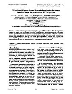
Figure 1: Statistical mean and three times the standard deviation of the calibrated data together with a lognormal fit. tograms could be resource intensive. Therefore we use theoretical models to parameterize the results. 0.03 Log−normal PDF fitting Calibration data statistics 0.025
0.02
PDF
In general, the goal of the calibration phase is to produce a mapping between the RSS of a packet and the distance between the receiver and the sender of that packet. In other words, we use the RSS as a method of ranging. However, in contrast to other ranging techniques (e.g., time-of-arrival of ultrasound waves), RSS is a very unreliable method of estimating the range from a transmitter, therefore, we will not seek a mapping from RSS to distance, but rather a mapping from RSS to a pdf of the corresponding distance. In an outdoor environment, the propagation is sufficiently predictable such that such a mapping is reasonably accurate. In this section we describe how we obtain this mapping. The calibration procedure is conceptually very simple: a transmitter and a receiver are placed at several (ideally many) known distances from each other and the RSS is measured (and logged) at the receiver for many packets. To make sure that several sources of errors are taken into account, several transmitter/receiver pairs should be used (to account for changes in the transmission power and receiver sensitivity), and during the calibration, the orientation of the pair should be changed to account for non-ideal radiation patterns of the antennas. For each distance a range or RSS measurements will be obtained. For calibration we used Compaq 3870 iPAQs with Lucent Orinoco cards [15]. Received Signal Strength Indicator (RSSI) data is measured every 2.5m up to 50m. For each distance we sent 1600 packets at different orientations of the sender and receiver and for each of these packets the receiver recorded the received signal strength in a database. We measured the signal strength by capturing each packet using the packet capture library (libpcap) and reading the data from the raw Orinoco header. RSSI is an arbitrary integer value corresponding to the power strength of the received packets measured by the wireless card. The mean and three times the standard deviation of the calibrated RSSI at each distance are shown in Fig. 1. The data shown in Fig. 1 corresponds to an environment free of any major obstacles (in the grass). We repeated the experiment in a heavily wooded area of our campus, and to our surprise, the results are very similar to the case of the environment free of obstacles. The data presented in Fig. 1 could be directly converted into histograms of distances corresponding to each RSS. One such normalized histogram (for RSSI=83) is shown in Fig. 2. However, storing and performing computations using the resulting his-
RSSI
100
0.015
0.01
0.005
0 0
5
10
15
20
25
30
Distance (m)
Figure 2: Log-normal distribution of distances for packets with RSSI=83. In general, the RSS P (in dB) at any fixed distance d is normally distributed, and the variance σP (d) does not vary significantly with the distance [22]. Let σP (d) ≈ σP , ∀d, then P[dB] = P(d)[dB] + XσP [dB], with
(1)
d ), (2) d0 where n is the path loss exponent, and the random variable XσP models shadowing effects and has a Gaussian distribution with zero mean and standard deviation σP . Both n and σP are dependent on the physical environment and can be determined from the calibration data; d0 is the close-in reference distance, and P0 is the RSS at d0 . Without loss of generality [22], we assume d0 = 1m. In Fig. 1, a log-normal shadowing model curve with n = 2.94 is also plotted to fit the calibration data. The exponent n is computed using logarithmic least square fitting. The RSS mean does not follow the fitting curve exactly, and the variance fluctuates as a function of the distance. Based on the log-normal model in equation (1), given a fixed RSS p, the distance D is log-normally P(d)[dB] = P0 [dB] − 10n lg(
ΨXC ,YC (x, y), which is a function of the coordinate random variable (XC ,YC );
distributed. Thereby, each RSS can be mapped uniquely to a pdf of D: p → lg D ∼ N(µD (p), σD (p)).
(3)
Both µD (p) and σD (p) can be determined from the calibration data as functions of the RSS p. Our outdoor calibration data shows that, given any RSS measurement, the pdf of D can be mapped log-normally as in equation (3). The mean µD (p) can be determined by considering the different probabilities of all the distances where RSS was equal to p: µD (p) = E(lg d|p). Similarly,p the standard deviation can be computed as σD (p) = Var(lg d|p). In Fig. 2 a log-normal mapping curve with mean µD (RSSI = 83) and standard deviation σD (RSSI = 83) fits well the experimental data, which indicates that the distance for RSSI=83 has indeed a log-normal distribution as predicted by the theoretical model.
• it updates the old pdf estimation by intersecting it with the generated constraint; and • finally, the unknown with the updated pdf estimation will broadcast to of all its neighbors. Assume an unknown j is within another node i’s transmission range and received a beacon packet with RSS pi, j dB. Unknown j maps pi, j to a pdf of the distance with mean µD (pi, j ) and standard deviation σD (pi, j ) as shown in equation (3); both µD (pi, j ) and σD (pi, j ) are calculated during the first phase. The unknown j then calculates a pdf constraint as:
ϕ (x, y) , ΨXC ,YC (x, y|pi, j ) = R ymax R xmax ymin xmin ϕ (x, y)dxdy ϕ (x, y) =
0.06
Z ymax Z xmax ymin
xmin
φ (x, y, xi , yi ) fXi ,Yi (xi , yi )dxi dyi , (5)
0.05
1 e φ (x, y, xi , yi ) = √ 2 2πσD (pi, j )di,2 j
−
0.04
PDF
(4)
0.03 0.02 0.01 0 40 90
30 85
20
80
10
Distance (m)
75 0
70
RSSI
Figure 3: The pdfs of distances for different RSSIs. In Fig. 3, the log-normal fitting curves for mappings from RSSI=70 to 90 are plotted. During the localization phase, these fitting curves are used to impose constraints on the position estimations of unknown nodes.
III.B. Phase II. Localization with Positive Constraints In this phase, each unknown estimates its position pdf, utilizing the log-normal mappings obtained in the first phase. Initially, each unknown sets its initial estimation to a uniform distribution over the entire network area, fX,Y (x, y) = A1 where A is the total area of the network. Nodes with position information, including both beacons and unknowns with updated pdf estimations, send out beacon packets to their neighbors. Upon receiving a beacon packet, an unknown executes the following algorithm: • it measures the RSS of the received beacon packet; • it maps the RSS to a one-dimensional pdf obtained in phase I and generates a pdf constraint
and
(lg di, j −µD (pi, j ))2 2 (p ) 2σD i, j
q di, j = (x − xi )2 + (y − yi )2 .
, (6)
(7)
where the constants xmin , xmax , ymin and ymax are the bounding coordinates of the network. Node i can be either a beacon or an unknown. Function fXi ,Yi (xi , yi ) is i’s position pdf estimate, which is a function of the coordinate variable (Xi ,Yi ). Variable di, j is the distance between nodes i and j. Specifically, if node i is a beacon and placed at (xb , yb ) (here we assume the position of the beacon is accurate, although the scheme may take into account any inaccuracies of the beacon’s position), the pdf estimate of beacon i can be represented as a two-dimensional Dirac’s delta function, (8) fXi ,Yi (xi , yi ) = δ 2 (xi − xb , yi − yb ). Assume the original pdf estimation for unknown j is fXold (x, y), and random variables (X j ,Y j ) and j ,Y j (XC ,YC ) are mutually independent; a new pdf estimation for unknown j can be calculated by intersecting the pdf constraint described above, either from a beacon or an unknown, with the original estimation. fXold (x, y)ΨXC ,YC (x, y|p) j ,Y j . fX j ,Y j (x, y) = R ymax R xmax old ymin xmin f X j ,Y j (x, y)ΨXC ,YC (x, y|p)dxdy (9) For example, Figure 4 depicts a network with three beacons (b1 , b2 , b3 ) and two unknowns (u1 , u2 ). First,
(a)
(b)
(c)
(d)
(e)
(f)
Figure 5: Localization evolution for the network topology in Fig. 4; (a) pdf estimation of u1 using beacon packets from b1 and b2 ; (b) pdf estimation of u2 using beacon packet from b3 ; (c) pdf constraint on u1 calculated by using u2 ’s beacon packet; (d) Final position estimate of u1 ; (e) pdf constraint on u2 calculated by using u1 ’s beacon packet; (f) Final position estimate of u2 . b1
b3 u1
u2
b2
Figure 4: An example of a network topology with three beacons (b1 , b2 , b3 ) and two unknowns (u1 , u2 ).
unknown u1 intersects its initial uniform pdf with two pdf constraints, which are obtained by using packets received from b1 and b2 . The newly computed pdf estimate is shown in Fig. 5(a). Similarly, unknown u2 generates a new pdf estimate using beacon packet from b3 as shown in Fig. 5(b). Consequently, both u1 and u2 send out beacon packets to their neighbors. When receiving the beacon packet from u2 , u1 calculates a pdf constraint as shown in Fig. 5(c); and it intersects this pdf constraint with its old pdf estimate in Fig. 5(a) to obtain its final position estimate as shown in Fig. 5(d). Unknown u2 , at the same time, carries the same sequence using u1 ’s beacon packet. Its newly computed pdf constraint and the final intersection are shown in Figs. 5(e) and 5(f). Intersection between the current position pdf estimation and the new constraint is only possible under the assumption of two vector random variables (X j ,Y j ) and (XC ,YC ) being mutually independent.
We will discuss how to combine the probabilities when dependencies occur (the realistic case) in Section IV.B. Therefore, the probability estimation of an unknown j being located at the coordinate (x j , y j ) is: Prob(x j , y j ) ≈
Z y j +∆y Z x j +∆x y j −∆y
x j −∆x
fX j ,Y j (x, y)dxdy. (10)
The probability Prob(x j , y j ) = Prob(X = x j ,Y = y j ). Both ∆x and ∆y are arbitrarily small values. The higher the probability Prob(x j , y j ), the more likely that the unknown node is located at (x j , y j ). The position of the unknown is thus determined at (x∗j , y∗j ) = arg max Prob(x j , y j ), x j ,y j
(11)
where xmin ≤ x j ≤ xmax and ymin ≤ y j ≤ ymax . In the above example, while the probability estimation for u1 has only one peak, which is at the true position of u1 . The probability estimation for u2 has two peaks, with the true position on the lower peak. To improve estimation accuracy and reduce uncertainty, negative constraints are introduced in the next section.
III.C. Phase III. Localization with Negative Constraints In this phase, we consider probabilistic negative constraints. In this enhancement, each unknown refines
its probability estimation using negative constraints. The negative constraint is defined as a function ρ (x, y) representing a constraint on an unknown when it cannot receive any packet from a given beacon. In other words, it is the information inferred by not hearing from a beacon. Assume for the moment there is no shadowing effect and the minimum acceptable RSS is Pmin (i.e., packets with RSS smaller than Pmin will not be received); if a beacon b is at (xb , yb ), an unknown j that is aware of beacon b’s position but unable to receive any of its packets computes a negative constraint which constrains itself outside the transmission range of beacon b; However, considering the shadowing effects (realistic case), the negative constraint can be calculated from calibration measurements. Recall that the RSS (in dB) at each distance is normally distributed as shown in equation (1). The negative constraint is then:
ρ (x, y) =
Z Pmin −∞
− 1 √ e 2πσP (db, j )
(p−P(db, j ))2 2 (d ) 2σP b, j
d p.
(12)
Thus, the probability estimate of unknown j is represented by the following probability: g y) = Prob(x,
Prob(x, y)ρ (x, y) . Prob(x, y)ρ (x, y) ∑xxmax ∑yymax min min
(13)
For example, using the same network topology in Fig. 4, node u2 can neither hear directly from b1 nor b2 . The intersection of b1 ’s and b2 ’s negative constraints is shown in Fig. 6(a). The final probability estimation for u2 after intersecting the old one with the negative constraint is shown in Fig. 6(b). For u2 ’s estimation, only one peak at the true position remains. In this case, the negative constraint refinement clearly helps to reduce the estimation uncertainty and improve the estimation accuracy compared to Fig. 5(f). We will evaluate the usefulness of negative constraints for more general settings in Section V.
(a)
(b)
Figure 6: Refinement using negative constraints. (a) The intersection of b1 ’s and b2 ’s negative constraints; (b) Final pdf estimation of u2 .
III.D. Reducing the Complexity
Computational
In order to implement the proposed approach, there are a number of ways to store and calculate the position estimates. In this paper, we use a uniform rectangular grid. The pdf estimations in the last section are replaced by probability mass functions (pmfs) estimation as the probability for an unknown being located in each square of the grid. Equations (4) and (5) become ΨXC ,YC (x, y|pi, j ) =
ϕ (x, y)
, ϕ (x, y)dxdy ∑xxmax ∑yymax min min
(14)
and
ϕ (x, y) =
ymax xmax
∑ ∑ φ (x, y, xi, yi ) fX ,Y (xi , yi )dxi dyi , i
i
(15)
ymin xmin
where both dx dy and dxi dyi approximate the area of a grid square. Both (XC ,YC ) and (Xi ,Yi ) are now discrete coordinate random variables. Equations (14) and (15) indicate that the proposed probabilistic approach can be computationally expensive. Wireless sensors usually have limited computational resources: a mica2 mote can compute and intersect two constraints in 15 seconds for a 100×100 grid [16]. It can be expected that the entire localization approach will take a few minutes; for most applications expecting months to years of service from the sensor network, this is a relatively small price to pay for accurate localization information. When approximating pdfs using rectangular grids there is a clear tradeoff between the precision and computational complexity: the finer the grid, the higher the precision and computational demands. If we assume the network deployment area is square and it is divided into an N × N uniform grid, the calculation for the pmf estimate for each unknown requires O(N 4 ) multiplication per operation. In order to reduce the computational complexity, we propose to use the Fast Fourier Transform (FFT), which is commonly used in digital signal processing. The variable φ (x, y, xi , yi ) in equation (15) is a function of (x − xi , y − yi ); therefore, the calculation of ϕ (x, y) is a two-dimensional discrete convolution:
ϕ (x, y) = φ (x, y) ⊗ fXi ,Yi (x, y).
(16)
Therefore, ϕ (x, y) can be calculated using the twodimensional FFT:
ϕ (x, y) = IFFT{FFT{φ (x, y)} × FFT{ fXi ,Yi (x, y)}}. (17)
In this way, the number of multiplications required is reduced to O(N 2 log2 N). The processing time can be further reduced if each node only computes constraints for the locations where its current position estimate is not zero - a very simple enhancement that can substantially reduce the computing time.
and the constraints cannot be performed. We classify the dependencies in two categories:
IV.
Figure 7: Network topologies with dependencies (node b is a beacon, all the others are unknowns): (a) i to i dependency case 1 (b) i to i dependency case 2 (c) common i constraint dependency.
Algorithm Design and Implementation
In this section, we will provide the details regarding the design of the algorithm that implements the ideas in Section III.
IV.A.
b
(a)
The only nodes providing accurate position information are beacons, and all unknowns estimate their position based on this information. In the proposed algorithm, each unknown stores a log as shown in Table 1. All entries start with a beacon identifier (IDb i) and the coordinates of the beacon (xb i, yb i). Each entry represents a transmission path from the beacon to the unknown node storing the log. IDu s are the IDs of the intermediate unknowns. A beacon can start multiple entries, as the first two entries shown in the table, since all of the neighboring unknowns of the beacon relay its position information. Similarly, a single unknown can appear in multiple entries. Upon the receipt of a log entry from a neighbor node (beacon or unknown), each unknown appends its node ID to the log entry and records the RSS of the received packet. Beacon packets from an unknown contain one or more entries from that unknown’s log. Packets from beacon nodes follow the same format (having only the beacon information).
m m2
j i
b
IV.B.1.
Packet and Log Format
m1
i
j
mk
(b)
b
i
j n
(c)
i to i dependency
Two typical cases of i to i dependency are shown in Figs. 7(a) and (b). In Fig. 7(a), after computing its pdf estimation fXi ,Yi (x, y) using packets from b, node i sends a beacon packet to unknown j. Unknown j, upon receiving the beacon packet, will recalculate its pdf estimate and broadcast the updates back to i. The new constraint calculated by i using the beacon packet sent by j is ΨXC ,YC (x, y|p j,i ), where p j,i is the RSS at i. It can be shown that (XC ,YC ) is dependent on (Xi ,Yi ). Fig. 7(b) shows another case with the same underlying dependency. Assume several unknowns (m1 , m2 , ..., mk ) are on a path between unknowns i and j. Assume that node i propagates a beacon packet on the path i → m1 → m2 → . . . → mk → j → i. Eventually, i will use the beacon packet from j to calculate constraint ΨXC ,YC (x, y|p j,i ). Just like in the case of in Fig. 7(a), (Xi ,Yi ) and (XC ,YC ) are dependent. In summary, the i to i dependency occurs in a path (log entry) where one unknown occurs more than once.
Table 1: Beacon packet format.
IV.B.2. Length Length Length . . .
IV.B.
IDb 1 IDb 1 IDb 2 . . .
xb 1 xb 1 xb 2 . . .
yb 1 yb 1 yb 2 . . .
IDu 11 IDu 21 IDu 31 . . .
RSS11 RSS21 RSS31 . . .
IDu 12 IDu 22 IDu 32 . . .
RSS12 RSS22 RSS32 . . .
··· ··· ··· . . .
Dependency Elimination
The log processing involves eliminating dependencies among different log file entries. Recall that when vector random variables (X j ,Y j ) and (XC ,YC ) are dependent, simple intersection between the pdf estimations
Common i constraint dependency
Fig. 7(c) shows a common i constraint dependency scenario. Both m and n update their pdfs using beacon packets from unknown i and broadcast their updates to unknown j. Assume the beacon packet from m arrives first, j updates its pdf to fX j ,Y j (x, y). Next j will use the beacon packet from n to calculate the pdf constraint ΨXC ,YC (x, y|pn, j ). Nevertheless, (Xm ,Ym ) and (Xn ,Yn ) are dependent, which results in the dependency between (X j ,Y j ) and (XC ,YC ). In the common i constraint dependency scenario, two or more paths share one or more intermediate unknowns.
From the discussion above, if each node appears only once in a single row of the log file, no i to i dependency exists. Therefore, the first kind of dependency can be eliminated by deleting all the rows, in each of which a node has been recorded multiple times. The common i dependency is eliminated by searching for all rows that contain the same intermediate unknown with different descendent unknowns. Among all these rows, the longer paths (in terms of hops) are deleted first. Among all remaining shortest paths, only one (randomly chosen) for every intermediate unknown is kept, others are discarded. This way the dependencies are eliminated. The estimation algorithm is repeated distributively at every unknown and, eventually, data from all beacon nodes will reach all the unknown nodes and the algorithm will stop. Alternatively, to reduce the number of messages, we can impose a lower threshold on the difference that has to occur in the position of an unknown for that node to forward a beacon packet: information from beacons after it travels many hops is often too diluted (i.e., the constraints, do not constrain too much) to make any difference in the position of a node. Therefore, the compute procedure at an unknown will stop after a relatively stable estimation is achieved.
V.
Simulation Results
Meaningful evaluation of the proposed approach is not trivial. We showed the practical feasibility of other (single hop and not considering negative information) probabilistic approaches [15, 16]. However, a practical experiment is limited with respect to the number of nodes and scenarios that can be considered. Therefore, we decided to evaluate the performance of our approach through simulations while using real world measurements for signal propagation models. Since standard networking issues (e.g., the routing algorithm, the transport layer, MAC fairness, etc.) do not affect the performance of our algorithm, we did not model the MAC, routing and transport layer. Instead we used Matlab to determine the signal strength between neighboring nodes (at the physical layer) and compute the constraints and position estimates (at the application layer). The results consider the precision (i.e., the uncertainty in the position estimates) and the accuracy (i.e., the difference between the real position of the nodes and the position determined by the localization algorithm) of the proposed approach. We compare the results with other well-known range-based localiza-
tion approaches (DV-distance [8] and multilateration [9, 23]). The precision of our approach is also compared with the Cramer-Rao lower bound (CRLB).
V.A.
Cramer-Rao Lower Bound
The CRLB is a lower bound which can be used to evaluate the variance of any unbiased estimator [24]. Assuming that there are M beacons and N unknowns in the network, let θ = [x1 , x2 , . . . , xN , y1 , y2 , . . . , yN ] be the coordinate variables to be estimated. The likelihood function is: f (lg d; θ ) =
M+N
∏ ∏ j=1
i∈H( j)
−
e
(lg di, j −lg d i, j )2 2 2σD
√
2πσD
,
(18)
i< j
where i ∈ H( j) means node i is within j’s transmission range. The CRLB can be calculated based on 2N × 2N Fisher Information matrix I(θ ) as shown in [25]. Therefore, variance of each estimated parameter is bounded from below:
σθ2i ≥ [I −1 (θ )]i,i . V.B.
(19)
Performance Evaluation
For the simulation we considered 50 unknowns and 6 beacons randomly placed in a square area (of variable size depending on the desired density). We used a rectangular grid with squares of 1m2 and imposed a threshold on the difference in position of 1m (i.e., unless the current estimated position is different by more than 1m from the previous position, the node does not rebroadcast the new information). The transmission radius was restricted to 13.5m (corresponding to an RSSI measurement of 78). We evaluated the effect of the variation of several parameters (number of hops the information is allowed to travel, density, number of unknowns, fraction of beacons and measurement inaccuracy), on the accuracy and the precision of the proposed approach. Unless otherwise specified, we used a node density of 0.03 nodes/m2 and a standard deviation for the RSS of 2.5 dB (corresponding to the value obtained from calibration measurements). For every graph we present the average of 20 simulations with different network topologies. All the results are normalized with respect to the transmission range.
V.B.1.
The Effect of the Number of Hops between Beacons and Unknowns
To evaluate the number of hops after which a beacon information becomes irrelevant we simulated the network and varied the number of hops that the beacon
Normalized average error
1.2 1 0.8 0.6 0.4 0.2
2
3
4
5
6
Number of hops n
(a)
7
8
9
10
4
Average beacon packets sent per node
0.01 0.015 0.02 0.025 0.03 0.04 0.05
1.4
0 1
Percentage of nodes at most n hops from a beacon
100
1.6
90
80
70
0.01 0.015 0.02 0.025 0.03 0.04 0.05
60
50
40 1
2
3
4
Number of hops n
5
(b)
6
3.5
3
0.01 0.015 0.02 0.025 0.03 0.04 0.05
2.5
2
1.5
1
0.5 2
3
4
5
6
7
Number of hops n
8
9
10
(c)
Figure 8: The Effect of the maximum number of hops between beacons and unknowns: (a) accuracy of the proposed approach as a function of the maximum number of hops from the beacons to the unknown nodes for different node densities; (b) the percentage of nodes reachable by at least one beacon in n hops as a function of the maximum number of hops from the beacons to the unknown nodes for different node densities; (c) the average number of packets sent by unknown nodes as a function of the maximum number of hops from the beacons to the unknown nodes for different node densities. packets are allowed to travel from the beacon nodes (similar to the time-to-live (TTL) field in IP). To eliminate the influence of measurement noise, we just ignored it in this simulation (but included it in all other simulations). The accuracy of the proposed approach as a function of the number of hops that beacon information is allowed to travel is shown in Fig. 8(a). Different lines correspond to different network densities. For sparse networks, many unknown nodes are unable to hear directly from the beacons, and, hence, have to rely on information propagated through multiple hops. Figure 8(a) shows that, regardless of the network density, information does not have to travel for many hops before the proposed approach converges: information from distant beacons cannot significantly improve the accuracy of the proposed approach. Thus, in the proposed approach unknown nodes only need local (a few hops away) information to localize themselves. Figure 8(b) shows the percentage of nodes that are within n hops range of at least one beacon for the same densities in Fig. 8(a). Figure 8(c) depicts the average number of packets sent by every unknown node for different network densities. Since each unknown broadcasts a beacon packet only after it has a considerable position improvement (larger than the threshold we set as 1m), the number of beacon packets required does not increase linearly with the limit on the number of hops. From the figure, we have two observations. First, more beacon packets are sent in high density networks when the allowed number of hops is small: more unknowns can hear directly from the beacons and forward the information. Second, for dense networks,
beacon packets with small TTL are enough for localization (as also shown in Fig. 8(a)); however, for low density networks, beacon packets from far away beacons may still affect the position estimate of an unknown. Therefore, more beacon packets are required to broadcast the change in the position estimates when the allowed number of hops is large. In what follows, all approaches are evaluated through two aspects: the accuracy (average estimation error) and the precision (standard deviation of the location estimate). For the proposed approach, results, both before and after the negative constraint refinement are shown in all the figures in order to highlight the influence of the negative constraints on the performance of the proposed system.
V.B.2.
The Effect of the Network Density
In this simulation we studied the effect of the network density on the accuracy of the proposed approach. To change the density we changed the deployment area and kept the number of beacons and unknowns constant. The accuracy and the precision results are presented in Figs. 9 and 10 respectively. Both the accuracy and the precision improve with the increase of the network density. This is not surprising as the CRLB is rather sensitive to the number of neighbors of a node. Similarly, in the proposed approach, the more neighbors, the more constraints will be placed on the unknowns. Another reason for the poor performance at lower densities is that (as shown in Fig. 8(b)) the unknowns are relatively too far from the beacon nodes to obtain any estimation improvements. The negative constraints improve the effectiveness of the proposed approach considerably: the per-
formance is very close to the optimum (the CRLB). 1.4 Positive constraint only Positive and negative constraint Multilateration DV_distance
Normalized average error
1.2
1
0.8
0.6
0.4
0.2
0 0.1
0.15
0.2
0.25
0.3
0.35
Density (node/m2)
0.4
0.45
0.5
Figure 9: The effect of network density on localization accuracy.
1.4 Positive constraint Positive and negative constraint Multilateration DV_distance CRLB
Normalized standard deviation
1.2
1
0.8
Second, we varied the number of the total nodes in the network from 30 to 100 while keeping the fraction of the beacons in the network as 10% and constant density. As can be seen from Figs. 11(b) and 11(e), the performances for the three phase probabilistic approach do not vary much along with the network scale, which obeys the tendency of the CRLB. Finally, to evaluate the effect of the beacon density on the proposed approach we varied the percentage of the beacons from 6% to 20%. The results are shown in Figs. 11(c) and 11(f). The CRLB indicates that the localization precision does not increase significantly with the increase of the beacon percentage. However, the precision of all approaches decreases for low beacon densities: at low beacon densities the packets from a beacon will take several hops to reach an unknown. In all algorithms, the estimation error is accumulated and propagated in each hop, which causes the relative poor performances for low beacon densities.
V.B.4.
The Effect of the Range Measurement Inaccuracy
0.6
0.4
0.8
0.2
Positive constraint only Positive and negative constraint Multilateration DV_distance
0.7 0.15
0.2
0.25
0.3
0.35 2
0.4
0.45
0.5
Density (node/m )
Figure 10: The effect of network density on localization precision.
Normalized average error
0 0.1
0.6 0.5 0.4 0.3 0.2 0.1
The Effect of The Number of Nodes
In this scenario, we varied the number of beacons and unknowns in three different ways. First, we varied the number of unknowns from 10 to 100 while maintaining the number of beacons and network density constant. The average errors and the standard deviation of the estimation are shown in Figs. 11(a) and 11(d) respectively. The standard deviation for all methods increase as the number of unknowns increases, while the CRLB is almost constant. The intuition behind this result is that only the beacon nodes are aware of their positions and introduce information into the system: the unknown nodes will estimate their positions based on the information from the beacons. As the number of unknowns increases, the numbers of hops from beacons to most of the unknowns increase as well (recall that the node density is kept constant), thus the information from the beacons will be diluted by going through multiple hops. The constant number of neighbors and beacons account for the almost constant CRLB.
0 0.5
1
1.5
2
2.5
3
3.5
4
Standard deviation σP of RSS (dB)
4.5
5
Figure 12: The effect of range inaccuracy on localization accuracy. 0.8 Positive constraint only Positive and negative constraint Multilateration DV_distance CRLB
0.7
Normalized standard deviation
V.B.3.
0.6 0.5 0.4 0.3 0.2 0.1 0 0.5
1
1.5
2
2.5
3
3.5
4
Standard deviation σP of RSS (dB)
4.5
5
Figure 13: The effect of range inaccuracy on localization precision. Finally, we studied the effect of the inaccurate measurements on the accuracy and the precision of the
0.9
0.8 Positive constraint only Positive and negative constraint Multilateration DV_distance
Positive constraint only Positive and negative constraint Multilateration DV_distance
0.6 0.5 0.4 0.3 0.2
Positive constraint only Positive and negative constraint Multilateration DV_distance
0.8
Normalized average error
0.6
Normalized average error
Normalized average error
0.7
0.5
0.4
0.3
0.7 0.6 0.5 0.4 0.3 0.2
0.2
0.1
0.1 20
30
40
50
60
70
80
90
0.1 30
100
Number of unknowns
40
50
(a)
70
80
90
0.6
0.7
0.3 0.2
0.1
30
40
50
60
70
Number of unknowns
(d)
80
90
100
20
0.4
0.2
20
18
0.5
0.3
0.1
16
0.6
0.4
0.2
14
Positive constraint only Positive and negative constraint Multilateration DV_distance CRLB
0.8
0.5
0.3
12
Percentage of beacons (%)
(c)
Positive constraint only Positive and negative constraint Multilateration DV_distance CRLB
0.7
0.4
0 10
10
0.9
Normalized standard deviation
0.5
8
(b)
Positive constraint only Positive and negative constraint Multilateration DV_distance CRLB
0.6
0 6
100
0.8
0.7
Normalized standard deviation
60
Number of nodes
Normalized standard deviation
0 10
0 30
0.1
40
50
60
70
Number of nodes
80
90
100
(e)
0 6
8
10
12
14
16
Percentage of beacons (%)
18
20
(f)
Figure 11: The Effect of The Number of nodes (a) The effect of the number of unknowns on localization accuracy (beacon number is constant) (b) The effect of the network scale on localization accuracy (beacon percentage is 10%) (c) The effect of beacon density on localization accuracy (d) The effect of the number of unknowns on localization precision (beacon number is constant) (e) The effect of the network scale on localization on localization precision (beacon percentage is 10%) (f) The effect of beacon density on localization precision. proposed approach, by increasing the standard deviation of the RSS (σP ). We varied σP between 0.5dB to 5dB (recall that the average σP from calibration measurements is approximately 2.5dB). The results are shown in Figs. 12 and 13. The CRLB increases proportionally to σP . The performance of all algorithms follows this increasing tendency, worsening their performance as the measurements become more inaccurate.
VI.
Conclusion
In this paper, we presented a distributed, RSS-based probabilistic localization approach for outdoor wireless sensor networks. The approach accounts for inaccurate range measurements by using probability functions for range measurements. Both positive and negative constraints originating at the beacons reduce the uncertainties of the positions of the unknown nodes. In order to reduce the computation complexity for fine estimation and large-scale networks, we also presented an extended probabilistic grid approach based on Fast Fourier Transform (FFT). The probabilistic approach is shown to outperform existing range-based localization approaches and approach the Cramer-Rao lower bound.
References [1] I. Akyildiz, W. Su, Y. Sankarasubramaniam, and E. Cayirci, “A survey on sensor networks,” IEEE Communication Magazine, vol. 40, no. 8, pp. 102–116, Aug. 2002. [2] P. Bahl and V. Padmanabhan, “RADAR: An in-building RF-based user location and tracking system,” in Proc. of IEEE INFOCOM 2000, vol. 2, Tel Aviv, Israel, Mar. 2000, pp. 775–584. [3] A. M. Ladd, K. E. Bekris, G. Marceau, A. Rudys, L. E. Kavraki, and D. Wallach, “Robotics-based location sensing using wireless ethernet,” in Proc. of ACM MobiCom 2002, Atlanta, Georgia, Sept. 2002. [4] J. Latvala, J. Syrj¨arinne, H. Ikonen, and J. Niittylahti, “Evaluation of RSSI-based human tracking,” in European Signal Processing Conference, 2000, pp. 2273–2277. [5] V. Bhargava and M. L. Sichitiu, “Physical authentication through localization in wireless local area networks,” in Proc. of IEEE Globecom 2005, St. Louis, MO, Nov. 2005.
[6] D. Madigan, E. Elnahrawy, R. P. Martin, W.H. Ju, P. Krishnan, and A. S. Krishnakumar, “Bayesian indoor positioning systems,” in Proc. of IEEE INFOCOM 2005, Miami, FL, Mar. 2005.
[16] M. L. Sichitiu and V. Ramadurai, “Localization of wireless sensor networks with a mobile beacon,” in Proc. of the First IEEE Conference on Mobile Ad-hoc and Sensor Systems (MASS 2004), Fort Lauderdale, FL, Oct. 2004.
[7] N. Priyantha, A. Chakraborthy, and H. Balakrishnan, “The cricket location-support system,” in Proc. of International Conference on Mobile Computing and Networking, Boston,MA, Aug. 2000, pp. 32–43.
[17] D. Niculescu and B. Nath, “Ad hoc positioning system (APS) using AOA,” in Proc. of IEEE INFOCOM 2003, Apr. 2003.
[8] D. Niculescu and B. Nath, “DV Based Positioning in Ad hoc Networks,” Telecommunication Systems, 2003. [9] A. Savvides, H. Park, and M. Srivastava, “The bits and flops of the n-hop multilateration primitive for node localization problems,” in First ACM International Workshop on Wireless Sensor Networks and Applications, Atlanta, GA, Sept. 2002. [10] C. Savarese, J. M. Rabaey, and J. Beutel, “Locationing in distributed ad-hoc wireless sensor networks,” in Proc. of ICASSP’01, vol. 4, 2001, pp. 2037–2040. [11] S. Capkun, M. Hamdi, and J. P. Hubaux, “GPSfree positioning in mobile ad-hoc networks,” Cluster Computing, vol. 5, no. 2, April 2002. [12] D. Moore, J. Leonard, D. Rus, and S. Teller, “Robust Distributed Network Localization with Noisy Range Measurements,” in Second ACM Conference on Embedded Networked Sensor Systems, Nov. 2004, pp. 50–61. [13] X. Ji and H. Zha, “Sensor Positioning in Wireless Ad-hoc Sensor Networks Using Multidimensional Scaling,” in Proc. of IEEE INFOCOM 2004, Mar. 2004, pp. 2652–2661. [14] A. Galstyan, B. Krishnamachari, K. Lerman1, and S. Pattem, “Distributed Online Localization in Sensor Networks Using a Moving Target,” in the third international symposium on information processing in sensor networks, 2004, pp. 61–70. [15] V. Ramadurai and M. L. Sichitiu, “Localization in wireless sensor networks: A probabilistic approach,” in Proc. of the 2003 International Conference on Wireless Networks (ICWN 2003), Las Vegas, NV, June 2003, pp. 275–281.
[18] R. Want, A. Hopper, V. Falco, and J. Gibbons, “The active badge location system,” ACM Transactions on Information Systems, vol. 10, pp. 91– 102, Jan. 1992. [19] N. Bulusu, J. Heidemann, and D. Estrin, “GPSless low cost outdoor localization for very small devices,” IEEE Personal Communications Magazine, vol. 7, pp. 28–34, Oct. 2000. [20] L. Doherty, K. S. J. Pister, and L. E. Ghaoui, “Convex position estimation in wireless sensor networks,” in Proc. IEEE INFOCOM 2001, vol. 3, Anchorage AK, Apr. 2001, pp. 1655– 1663. [21] T. He, C. Huang, B. M. Blum, J. A. Stankovic, and T. Abdelzaher, “Range-Free Localization Schemes for Large Scale Sensor Networks,” in Proc. of ACM MobiCom 2003, 2003, pp. 81–95. [22] T. S. Rappaport, Wireless Communications: Principles and Practice, 2nd ed. Pearson Education, 2001. [23] A. Savvides, C. C. Han, and M. B. Srivastava, “Dynamic fine-grained localization in adhoc networks of sensors,” in Proc. of ACM Mobicom 2001), Rome, Italy, July 2001, pp. 166– 179. [24] S. M. Kay, Fundamentals of Statistical Signal Processing, Volume I: Estimation Theory, 1st ed. Prentice Hall, 1993. [25] N. Patwari, A. O. Hero, M. Perkins, N. S. Correal, and R. J. O’dea, “Relative Localization Estimation in Wireless Sensor Network,” IEEE Transactions on Signal Processing, vol. 51, pp. 2137–2148, Aug. 2003.