A PROBABILITY-ESTIMATION-BASED STRATEGY TO OPTIMIZE THE CLASSIFICATION RULE SET EXTRACTED FROM BAYESIAN NETWORK CLASSIFIERS Glaucia M. Bressan∗, Vilma A. Oliveira∗, Estevam R. Hruschka Jr.†, Maria C. Nicoletti† ∗
Universidade de S˜ ao Paulo Depto. de Engenharia El´etrica Av. do Trabalhador S˜ ao Carlense, 400 S˜ ao Carlos, SP, Brasil †
Universidade Federal de S˜ ao Carlos Depto. de Computa¸ca ˜o S˜ ao Carlos, SP, Brasil
Emails:
[email protected],
[email protected],
[email protected],
[email protected] Abstract— This paper describes the modeling of a biomass-based weed-crop competitiveness classification process based on classification rules extracted from Bayesian network classifiers. Two Bayesian network classifiers are employed, namely an unrestricted Bayesian network classifier and a na¨ıve Bayes classifier. The BayesRule algorithm is then used to extract a set of rules from each Bayesian network classifier. In the sequel, the class probability estimate is used as a pruning strategy to optimize each rule set. Results concerning the performance and adequacy of the proposed pruning strategy are presented and discussed for comparison purposes. Resumo— Este trabalho descreve a modelagem de um processo de classifica¸ca ˜o da competitividade entre plantas daninhas e cultura considerando a biomassa das plantas. O processo ´ e baseado em regras extra´ıdas de redes Bayesianas de classifica¸ca ˜o. Duas redes Bayesianas de classifica¸ca ˜o s˜ ao empregadas, sendo uma rede de classifica¸ca ˜o Bayesiana irrestrita e uma rede na¨ıve Bayes. O algoritmo BayesRule ´ e ent˜ ao usado para extrair um conjunto de regras a partir de cada uma das redes. Em seguida, a estimativa da probabilidade da classe ´ e usada como estrat´ egia de poda para otimizar cada conjunto de regras. Resultados referentes ao desempenho e adequa¸ca ˜o da estrat´ egia de poda proposta s˜ ao apresentados e discutidos para fim de compara¸ca ˜o.
1
Introduction
Agricultural procedures may modify the ecological balance due to the way the growers till the land, leading to a population explosion (infestation) of some inconvenient plants, called weeds (Shiratsuchi, 2001). Dynamic models indicate that infestation is not only dependent upon the weed density but also upon the competitiveness of the weed species (Park et al., 2003; Firbank and Watkinson, 1985; Kropff and Spitters, 1991). More recently, competitive indices and weed ranking were used to quantify the weed competitiveness in a soybean field (Hock et al., 2006). Statistics-based classification methods have been considered for a long time in many research areas. These methods are based on probabilities that a given set of measurements come from objects belonging to a certain class. Using the performance of a na¨ıve Bayes classifier as a selection criterion, Granitto et al. (2002) describe experiments that identified a nearly optimal set of 12 seed characteristics to be used as classification parameters, which include coloration, morphological and textural features. Considering the seed identification problem, the work described in Granitto et al. (2005) compared the performance of a na¨ıve Bayes classifier versus an artificial neural networkbased (NN) classifier. In this particular experiment the na¨ıve Bayes classifier with an adequately
selected set of classification features outperformed the NN-based classifier. Similar results were also obtained by experiments discussed in Marchant and Onyango (2003) for a task of discrimination among plant, weed and soil. The knowledge represented by a Bayesian classifier is not as understandable as some other forms of knowledge representation, such as classification rules. Trying to circumvent this difficulty, a method called BayesRule proposed in Hruschka et al. (2007), uses the concept of maximum a posteriori (MAP) probability to extract a set of probabilistic rules that describes the classification task. In addition, the Markov blanket concept is applied to reduce the number and the complexity of classification rules generated by the extraction process. The BayesRule method was successfully used for translating a Bayesian classifier into a set of linguistic probabilistic rules in the work described in Bressan et al. (2007). The Bayes classifier was constructed aiming at the automatic classification of the degree of competitiveness among weeds and corn-crop. In this specific weed-crop competitiveness classification task, however, the Markov blanket concept was not sufficient to prune the rule set extracted from the Bayesian network classifier. In this sense, this paper proposes, implements and discusses a new pruning strategy to optimize a rule set created by the BayesRule method. A Bayesian
network classifier built using human expert knowledge (as described in Bressan et al. (2007)) and a na¨ıve Bayes classifier are used as input to the rule extraction process and then the proposed pruning strategy is applied to both rule sets. The results are analyzed and compared. The remaining of this paper is organized as follows. Section 2 describes the basics of Bayesian networks and na¨ıve Bayes classifiers. Section 3 initially describes the crop as well as the procedures used for collecting the data. In the sequence, it discusses how the BayesRule approach operates. Section 4 presents the results using both an unrestricted Bayesian Network classifier and a na¨ıve Bayes classifier as input to BayesRule. Finally, Section 5 presents some concluding remarks and highlights the next steps of this research work. 2
Bayesian Networks and Na¨ıve Bayes Classifiers
An unrestricted Bayesian network (Cheng et al., 2002), or simply Bayesian network for short, has a directed acyclic graph structure. Each node in the graph corresponds to a discrete random variable in the knowledge domain. An edge Y −→ X in the graph describes a parent-child relation, where Y is the parent and X is the child. All parents of X define the parent set of X. Each node of the Bayesian network structure is associated to a conditional probability table that specifies the probability of each possible state of the node, given each possible combination of states of its parents. If a node has no parents, its conditional probability table gives the marginal probabilities of the variable it represents. Thus, a Bayesian network represents a joint probability distribution over a set of random variables and can be used to make inferences on any node. Instead of encoding a joint probability distribution over a set of random variables, a Bayesian network classifier aims at predicting the value of a discrete class variable, given the value of a vector of features variables. Bayesian Networks can also be used as classifiers; this is done in this work. The learning of an unrestricted Bayesian network is a two-step process. First, the structure of the network is learnt and then its numerical parameters are learnt. A Bayesian network, however, is not designed to optimize the conditional likelihood of the class given the other features (Domingos and Pazzani, 1997). As a consequence, Bayesian networks may not produce good classification results. Actually, even the na¨ıve Bayes classifier (Friedman et al., 1997) can outperform more complex Bayesian networks classifiers in some domains. For this reason, in this paper, both, an unrestricted Bayesian network classifier and a na¨ıve Bayes classifier are used in the conducted experiments, for comparison purposes.
A na¨ıve Bayes is a special case of an unrestricted Bayesian network. In particular, it is a Bayesian network in which the class node has no parents. Also, each feature has the class node as its unique parent. The structure of a na¨ıve Bayes is fixed, that is, it is not necessary to learn a na¨ıve Bayes structure from data. Consequently, only the numerical parameters of the model need to be learnt, thus only information about the features and their corresponding values are needed to estimate probabilities. The computational time complexity of learning a na¨ıve Bayes network is linear with respect to the amount of training instances. The construction is also space efficient, requiring only the information provided by two-dimensional tables, in which each entry corresponds to a probability estimated for a given value of a particular feature. However, the na¨ıve Bayes method makes a strong and unrealistic assumption: all the features are conditionally independent given the value of the class. 3
Weed-crop Competition Classification
This section initially details how the weed-crop data was collected, prepared and used in the experiments. Next, it describes the process for constructing and evaluating two Bayesian networks, the unrestricted and the na¨ıve. The second subsection focuses on the process of extracting linguistic rules from both previously constructed Bayesian networks, using the BayesRule method proposed in Hruschka et al. (2007). 3.1
Collecting and Preparing the Weed-Crop Data
In the experiments described in this paper, data from a corn-crop field located in an experimental farm of the Empresa Brasileira de Pesquisa Agropecu´aria (Embrapa), in Sete Lagoas, Minas Gerais, Brazil is used 1 . The field was tilled in a 49ha area in 16 - 20 November 2004 and in 15 19 May 2006. The area contains 41 experimental field parcels 100 meters distant from each other. The parcels have a rectangular shape measuring 4 meters in the east-west direction and 3 meters in the north-south direction with 5 corn rows separated from each other by 0.7m, starting 0.1m from the bottom border. Before the crop development, glifosate 2.4kgha−1 herbicides were applied out of the parcels. Also, after the crop development, nicosulfuron 0.04kgha−1 and atrazine 1kgha−1 were applied. At the time of the application of herbicides, the parcels were covered. 1 Embrapa - Project 55.2004.509.00. Rede de Conhecimento em Agricultura de Precis˜ ao para Condi¸co ˜es do Serrado e dos Campos Gerais.
A weed can be more (or less) competitive with the crop depending on the type of its leaves. Therefore, the features for the Bayesian network classifier were selected as the total density of weeds per parcel, that is, the number of weeds per m2 , and the corresponding proportions of narrow and broadleaf weeds. The class variable is the weed biomass, which is defined as the amount of dry material per m2 of the aerial part of the weeds. The higher the biomass of a weed, the higher its competitiveness. To obtain the weed density data per m2 in each parcel, 4 squares of 0.5m × 0.5m were randomly placed within each parcel and the weed species of narrow-leaf and broadleaf were collected and counted. The weed species were separated into bags and kept in a greenhouse at the temperature of 1050 C until their weight become constant. At this point, the biomass of the species is measured. The density and the biomass measurements were collected in each experimental field parcel in April 2005 and October 2006, in two different corn-crops. Therefore, 82 data instances were obtained, that is, two data instances for each one of the 41 parcels. Analyzing the collected data, 11 data instances were identified as outliers and removed; the remaining 71 data instances were considered for inducing and evaluating two networks, an unrestricted Bayesian and a na¨ıve Bayes classifier. In order to evaluate each network a 10-fold cross validation process was adopted. 3.2
Table 1: Discretizing intervals for the features. Total density Narrow leaf density Broadleaf density Biomass
High [0.60,1] [0.60,1] [0.75,1] [0.60,1]
Low [0,0.20] [0,0.20] [0,0.25] [0,0.20]
Medium ]0.20,0.60[ ]0.20,0.60[ ]0.25,0.75[ ]0.20,0.60[
Figure 1: Biomass inference. node identified as Biomass is the class node, from which the competitiveness is inferred. The Markov blanket of this node is formed by all the variables of the Bayesian network classifier. Figure 3 illustrates the na¨ıve Bayes network structure, in which the class variable has no parents and the features are conditionally independent, given the class variable.
Bayesian Network Modelling
As mentioned in the Introduction, the knowledge represented by a Bayesian classifier is not easily understood by human beings. A way of promoting its understandability is by translating it into a more suitable representation, such as classification rules. A standard propositional if-then classification rule is the simplest and most comprehensive way to represent classification knowledge and, for this reason, this type of rule has been adopted by the BayesRule method. The BayesRule method (Hruschka et al., 2007) implements the translation process. In order to extract probabilistic rules from both previously built networks, using the BayesRule approach, the values of all the variables needed to be discretized. The discretizing process was conducted by a human expert who proposed three intervals as shown in Table 1, represented by the linguistic variables: low (L), medium (M) and high (H). Figure 1 represents the classifier system for the weed-crop competitiveness using the rule set extracted from either (unrestricted or na¨ıve) Bayesian network. Figure 2 illustrates the Bayesian network classifer structure defined by a human expert represented by the parent-children relationships. The
Figure 2: The Bayesian network classifier. As mentioned before, each node of a Bayesian network classifier has an associated set of conditional probabilities, that depends on its parents. Using a 10-fold cross validation process, 10 Bayesian networks were trained using 10 different training sets and the extracted rules were evaluated using each of the 10 corresponding testing sets. The same testing sets were used to evaluate the extracted rules from both networks, unrestricted and na¨ıve. The network structure, as shown in Figure 2, was constructed based on human knowledge about this particular domain. To circumvent the difficulties in estimating the conditional probabilities distribution from data, the Genie 2 , a free software, was used. 2 http://genie.sis.pitt.edu
4
Figure 3: The na¨ıve Bayes classifier.
The BayesRule algorithm for extracting classification rules from a Bayesian classifier which has been customized for this particular experiment is described in Algorithm 1. In the algorithm, the three variables, JBL , JN L and JT otal are initialized with value 3, representing the number of possible values these variables can have, that is, High, Medium and Low. The variables VBL , VN L and VT otal are 3-dimensional vectors containing all possible values these variables can have, again, High, Medium and Low. RI is a variable used to control and identify the number of rules that will be extracted from the Bayesian network classifier. Algorithm 1 (Procedure BayesRule) input: BC: Bayesian Classifier with 4 nodes {Figure 2} Biomass: Class variable output: SR {Set of Rules } begin 1. SR ← ∅ 2. CM B ← M B(Biomass) {Markov blanket of Biomass} 3. JBL ← 3 4. JN L ← 3 5. JT otal ← 3 6. VBL ← [High, Low, Medium] 7. VN L ← [High, Low, Medium] 8. VT otal ← [High, Low, Medium] 9. RI ← 1 {Rule Index} 10. for k2 := 1 to JBL do for k3 := 1 to JN L do for k4 := 1 to JT otal do begin {create rule antecedent } propagate rule antecedent throughout BC, determine Biomass value V alBio and define rule RRI as: if DensBL=vBLk2 and DensNL=vN Lk3 and DensTotal=vT otalk4 then Biomass = V alBio SR ← SR ∪ {RRI }; RI ← RI + 1 end 11. SR ← remove-irrelevant-rules(SR) end
Bayesian Network and Na¨ıve Bayes Classifiers Results
BayesRule extracted a set of 27 probabilistic rules from each Bayes classifier. The number of rules represents all the combinations of the variables and their linguistic variables. Each rule has a value that represents the probability of its class value, given the values of its antecedent variables. In order to reduce the number of rules in each rule set, a pruning strategy was used. Using each one of 10 cross validation training sets, the rules with probability less than 0.7 were replaced by a default rule, which was generated from an a priori probability of the class variable, obtained from the numerical parameters of the network. In this work, the most probable value for the class variable is the Medium linguistic value. Considering that a 10-fold cross validation strategy was used in the experiments, only one of the 10 testing set was chosen to be shown for each classifier; the results of the nine other testing sets were similar. Considering the Bayesian rules set extracted from the unrestricted Bayesian classifier, the results obtained for the mentioned testing set including the accuracy and the corresponding class probability are shown in Table 2. The rules are 50% in agreement with the testing set, since 3 out of 6 data instances were correctly classified. Table 3 shows the pruned Bayesian rule set, which presents rules with probability larger than 0.7 as well as the default rule. Table 4 shows the results of the testing set using the pruned rule set of Table 3. For this testing set, rules 9 and 21 were replaced by the default rule and the pruned rule set was 83.33% in agreement with the testing set, since 5 out of 6 instances were correctly classified. In this particular modeling, the classification rate has improved. For all the 10 testing set cases, the 71 data instances were tested. The results indicate 63.39% of agreement, since 45 of 71 testing data were correctly classified. By replacing the rules with probability less than 0.7 by the default rule, this percentage becomes 64.79%, since 46 out of 71 testing instances were correctly classified. Table 2: Unrestricted Bayesian network testing data set results. DensBL DensNL TotalDens Biomass rule Test Prob. H M M H 9 incorrect 52% M H M M 21 incorrect 55% H L M M 6 correct 71% H L M M 6 correct 71% H M M M 9 incorrect 52% M M L L 26 correct 80%
Table 5 shows the results for one testing set when considering the Bayesian rule set extracted from the na¨ıve Bayes classifier. The results reveal
Table 3: Pruned unrestricted Bayesian rule set. D:
Table 5: Na¨ıve Bayes testing data set results.
Default rule DensBL DensNL TotalDens Biomass rule Test Prob. H M H H 3 incorrect 62% 1 If (DensBL is H) and (DensNL is H) and (TotalDens is H) L H L M 13 correct 52% then Biomass is H (0.72) M M M M 27 correct 48% 4 If (DensBL is H) and (DensNL is L) and (TotalDens is H) M H M M 25 incorrect 50% then Biomass is M (1.00) M M M M 27 correct 48% 6 If (DensBL is H) and (DensNL is L) and (TotalDens is M) H L M L 20 incorrect 91% then Biomass is M (0.72) 7 If (DensBL is H) and (DensNL is M) and (TotalDens is H) then Biomass is H (0.83) 11 If (DensBL is L) and (DensNL is H) and (TotalDens is L) Table 6: Pruned na¨ıve Bayes rule set. D: Default rule then Biomass is M (1.00) 19 If (DensBL is M) and (DensNL is H) and (TotalDens is H) then Biomass is L (1.00) 2 If (DensBL is H) and (DensNL is L) and (DensdTotal is H) 23 If (DensBL is M) and (DensNL is L) and (TotalDens is L) then Biomass is M (0.80) then Biomass is L (0.79) 5 If (DensBL is L) and (DensNL is L) and (DensdTotal is H) 24 If (DensBL is M) and (DensNL is L) and (TotalDens is M) then Biomass is M (0.73) then Biomass is L (0.72) 18 If(DensBL is M) and (DensNL is M) and (DensdTotal is L) 26 If (DensBL is M) and (DensNL is M) and (TotalDens is L) then Biomass is L (0.71) then Biomass is L (0.80) 19 If (DensBL is H) and (DensNL is H) and (TotalDens is M) 27 If (DensBL is M) and (DensNL is M) and (TotalDens is M) then Biomass is M (0.76) then Biomass is M (0.80) 20 If (DensBL is H) and (DensNL is L) and (TotalDens is M) D otherwise Biomass is M (1.00) then Biomass is M (0.91) 21 If (DensBL is H) and (DensNL is M) and (TotalDens is M) then Biomass is M (0.78) 23 If (DensBL is L) and (DensNL is L) and (TotalDens is M) Table 4: Unrestricted Bayesian network testing data then Biomass is M (0.85) set results using the pruned rule set. D: Default rule D otherwise Biomass is M (1.00) DensBL DensNL TotalDens Biomass rule H M M H D M H M M D H L M M 6 H L M M 6 H M M M D M M L L 26
Test incorrect correct correct correct correct correct
Prob. 100% 100% 71% 71% 100% 80%
that the rules are 50% in agreement with the testing set, since 3 out of 6 instances were correctly classified. Table 6 shows the pruned Bayesian rule set and Table 7 shows the results of the testing set using the pruned rule set. For this testing set, rules 3, 13, 25 and 27 were replaced by the default rule and the pruned rule set was 66.66% in agreement with the testing set, since 4 out of 6 data instances were correctly classified. In this particular modelling, the classification has also improved. For all the 10 testing set cases, the 71 data instances were tested. The results using the unpruned rule set indicate 57.75% of agreement, since 41 of 71 testing data were correctly classified. By replacing the rules with probability less than 0.7 by the default rule, this percentage increases to 61.97%, since 44 out of 71 testing instances were correctly classified. 5
Conclusions
In this work two Bayesian weed-crop competitiveness models, based on weed biomass, are constructed aiming at extracting standard propositional if-then classification rules and a rule pruning strategy is proposed. The first model was
built using the concept of unrestricted Bayesian network classifier and the second is a traditional na¨ıve Bayes classifier. The numeric parameters of both Bayesian models were learned from the 71 data instances collected from a corn-crop. A hybrid approach, implemented by the BayesRule method, which articulates Bayes and linguistic rules was used to improve the model understandability, by extracting classification rules from each model. After the extraction process, the proposed rule pruning strategy was applied and a pruned Bayesian rule set was obtained (for each model) containing only rules with probability larger than 70%. By using the pruned rule set in both classifiers, the classification accuracy of the competitiveness, inferred from the weed biomass, increased and the number of rules decreased. Moreover, the proposed pruning strategy is promising since the resulting Bayes rule set translates the specialist knowledge. In addition, the results reveal that the unrestricted Bayesian classifier (induced with a human expert help) yields a higher agreement percentage than the na¨ıve Bayes classifier. The strong and unrealistic assumption (that all the features are independent given the class) which is an intrinsic aspect of any na¨ıve Bayes classifier may have contributed to this behavior. Although the measurements refer to a particular domain, it is important to mention that the results are specific to a particular crop field, subject to the conditions described in Subsection 2.1. Further work includes the use of extensive simu-
Table 7: Na¨ıve Bayes testing data set results using the pruned rule set. D: Default rule DensBL DensNL TotalDens Biomass rule Test H M H H D incorrect L H L M D correct M M M M D correct M H M M D correct M M M M D correct H L M L 20 incorrect
Prob. 62% 100% 100% 100% 100% 91%
lations and experiments trying to generalize the obtained results. It is intended also to investigate the proposed pruning strategy in other domains to confirm its relevance. Acknowledgements This work was partially supported by the Coordena¸c˜ao de Aperfei¸coamento de Pessoal de N´ıvel Superior (CAPES) under the Programa Nacional de Coopera¸c˜ao Acadˆemica (PROCAD), the Conselho Nacional de Desenvolvimento Cient´ıfico e Tecnol´ ogico (CNPq) and Funda¸c˜ao de Amparo `a Pesquisa do Estado de S˜ao Paulo (FAPESP). We thank Dr. D´ecio Karam from Embrapa Milho e Sorgo, Sete Lagoas, MG, for helping to define the Bayesian network structure and for providing the data used in the experiments described in this paper. References Bressan, G. M., Oliveira, V. A., Hruschka, E. R. J. and Nicoletti, M. C. (2007). Biomass based weed-crop competitiveness classification using Bayesian networks, 7th International Conference on Intelligent Systems Design and Applications . (accepted). Cheng, J., Greiner, R., Kelly, J., Bell, D. and Liu, W. (2002). Learning Bayesian networks from data: an information-theory based approach, Artificial Intelligence 137(1): 43–90. Domingos, P. and Pazzani, M. (1997). On the optimality of the simple Bayesian classifier under zero-one loss, Machine Learning 29(23): 103–130. Firbank, L. G. and Watkinson, A. R. (1985). A model of interference within plant monocultures, Journal of Theoretical Biology 116(2): 291–311. Friedman, N., Geiger, D. and Goldszmidt, M. (1997). Bayesian network classifiers, Machine Learning 29(2-3): 131–163. Granitto, P. M., Navone, H. D., Verdes, P. F. and Ceccatto, H. A. (2002). Weed seeds identi-
fication by machine vision, Computers and Electronics in Agriculture 33(2): 91–103. Granitto, P. M., Verdes, P. F. and Ceccatto, H. A. (2005). Large-scale investigation of weed seed identification by machine vision, Computers and Electronics in Agriculture 47(1): 15–24. Hock, S. M., Knezevic, S. Z. and Martin, A. (2006). Soybean row spacing and weed emergence time influence weed competitiveness and competitive indices, Weed Science 1(54): 38–46. Hruschka, E. R. J., Nicoletti, M. C., Oliveira, V. A. and Bressan, G. M. (2007). Markovblanket based strategy for translating a Bayesian classifier into a reduced set of classification rules, Proc. of the 7th Hybrid Intelligent Systems . (accepted). Kropff, M. J. and Spitters, C. J. T. (1991). A simple model of crop loss by weed competition from early observations on relative leaf area of the weeds, Weed Research 2(31): 97–107. Marchant, J. A. and Onyango, C. M. (2003). Comparison of a bayesian classifier with a multilayer feed-forward neural network using the example of plant/weed/soil discrimination, Computers and Electronics in Agriculture 39(1): 3–22. Park, S. E., Benjamin, L. R. and Watkinson, A. R. (2003). The theory and application of plant competition models: an agronomic perspective, Annal of Botany 92(6): 741–748. Shiratsuchi, L. S. (2001). Mapeamento da Variabilidade Espacial das Plantas Daninhas com a Utiliza¸ca ˜o de Ferramentas da Agricultura de Precis˜ ao, Master’s thesis, Escola Superior de Agricultura Luiz de Queiroz, Universidade de S˜ao Paulo, Piracicaba, SP.