are carried out with a legacy code written in C, developed in our group [16]. .... Succi, S.: The Lattice Boltzmann Equation: for Fluid Dynamics and Beyond. Nu-.
A Problem Solving Environment for Modelling Stony Coral Morphogenesis Roeland Merks, Alfons Hoekstra, Jaap Kaandorp, and Peter Sloot University of Amsterdam, Section Computational Science, Kruislaan 403, 1098 SJ Amsterdam, The Netherlands {roel,alfons,jaapk,sloot}@science.uva.nl, WWW home page: http://www.science.uva.nl/research/scs
Abstract. Apart from experimental and theoretical approaches, computer simulation is an important tool in testing hypotheses about stony coral growth. However, the construction and use of such simulation tools needs extensive computational skills and knowledge that is not available to most research biologists. Problem solving environments (PSEs) aim to provide a framework that hides implementation details and allows the user to formulate and analyse a problem in the language of the subject area. We have developed a prototypical PSE to study the morphogenesis of corals using a multi-model approach. In this paper we describe the design and implementation of this PSE, in which simulations of the coral’s shape and its environment have been combined. We will discuss the relevance of our results for the future development of PSEs for studying biological growth and morphogenesis.
1
Introduction
During its development, the three-dimensional shape of an organism is unfolded, guided by the genetic information stored in the DNA. To understand this process, called morphogenesis, it is very important to unravel the physical mechanisms underlying it [1]. Apart from experimental and theoretical approaches, during the last decenniums computational approaches have become more and more important in the study of morphogenesis [2,3]. We have applied computational models to understand the morphogenesis and environmental plasticity of stony corals (see e.g. [4,5,6,7,8,9]). In these models, a computational model of the growing coral was combined with a model of the physical environment. Developing and using the tools needed for such computational studies needs extensive training and knowledge that is not widely available to research biologists. Computational studies are therefore often carried out by mathematicians, physicists, computer scientists or computationally trained biologists, who inevitably spend a major part of their time in code and algorithm development. Problem solving environments (PSEs) [10,11] are software systems aiming to alleviate this issue. They hide the implementation details of a simulation code and allow the user to formulate her or his problem at a higher abstraction level, in the language of the problem being studied. Moreover, PSEs should contain
2
some knowledge about the simulation system, in order to be able to advise the user about the chosen parameters and warn him or her when necessary. PSEs should make it possible to separate the technical work on the simulation codes and methods from the conceptual computational experimentation and analysis. In this paper we will describe a prototypical PSE for the study of coral morphogenesis in interaction with the physical environment. In this PSE the problem can be formulated in high-level terminology. Boundary conditions and initial conditions are made available as independent modules, enabling easy specification of the simulation set-up. The modular architecture encourages a multi-model approach, were different models and solving methods can easily be tested and compared. In Section 2 the problem set covered by the PSE will be shortly described. In Section 3 we will describe the software architecture of the PSE, and discuss some of its results. Finally, in Section 4 we will discuss the relevance of our results for the simulation of morphogenesis.
2
Model and Methods Covered by the PSE
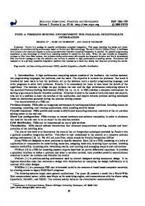
The coral growth PSE enables experimentation with several models of coral morphogenesis. These models can be roughly divided into two classes, the aggregation [4,5] models and the accretion [6,7,8,9] models. The aggregation models are based on the diffusion-limited aggregation (DLA) model as introduced by Witten and Sander [12]. In the DLA model an initial solid seed is placed in an (n-dimensional) simulation box. A particle, carrying out a random walk, is released until it hits a solid particle to which it attaches irreversibly. This procedure is iterated until an aggregate has formed. In an extension of this model, the particles are transported both by advection and by diffusion (advection-diffusion limited aggregation: ADLA). This model was studied by Kaandorp et al. [4,5] as a model of coral growth under the influence of fluid flow. In the accretion models, growth occurs as the iterative construction of layers, represented by triangulated meshes. In contrast to the aggregation models, in these models growth occurs in parallel all over the surface. This iterative accretive construction can be considered either a discrete (e.g. seasonal) process or the discretisation of a continuous growth process. The local thickness of the accreted layers can depend on a number of factors, such as the availability of a nutrient in the surrounding water [6], transported by advection-diffusion. This model is called the hydrodynamically influenced radiate accretive growth (HIRAG) model, and was reassessed in a more recent paper [7]. In the polyp oriented radiate accretive growth (PORAG) model, the individual polyps contributing to the growth process are explicitly taken into account [8,9]. Both the HIRAG and PORAG models have been included in the coral growth PSE. In Fig. 1 we present a flow diagram of these accretive coral growth models. The simulations are carried out partly in parallel, as indicated by the decomposed computational grids. The initial condition is formed by an initial geometry and a set of parameters (I). The next two stages, the dispersion of nutrients through flow and diffusion, take up the majority of the computational time (data
3
para− meters
I
II
III
sequential step
V
next growth cycle
IV
g
output for analysis and visualisation
Fig. 1. Flow diagram of the accretive coral growth models, consisting of five modules. I. Initial condition. II. Flow calculation. III. Advection-Diffusion IV. Flux measurements. V. Accretion. The modules I and V are replaced for (parallel) modules to obtain the aggregation model.
not shown); therefore this part of the simulation is carried out in parallel. The initial geometry is voxelised and divided over all the processors. If desired, a stable, laminar flow field is calculated (II) using the lattice Boltzmann BGK method [13]. After this, the advection-diffusion equation is solved using the moment propagation method [14,15], until a sufficiently stable field has been obtained. Finally, the nutrient fluxes are measured at a number of points scattered over the growing geometry (IV). These flux measurements are sent back to the master processor to carry out a growth step. The growth function g determines the thickness of the new growth layer based on these nutrient fluxes and possibly on the measurements of the local curvature of the latest geometry. The new geometry is the input of the next growth cycle. A more detailed description of these models is given elsewhere [7,8,9]. The structure of the aggregation models
4
Fig. 2. Results of the models covered by the PSE. a-b) Accretion models: a) Hydrodynamically influenced radiate accretive growth (HIRAG) model b) Polyp Oriented Radiate Accretive Growth (PORAG) model. Gray scale indicates nutrient flux, white: high flux, black: low flux c) Aggregation model. Cross sections of three dimensional simulations. Gray scale indicates resource concentration only partially differs from the accretion models. The geometric description of the morphology is absent, instead the growth form is represented by a cluster of solidified lattice sites. The initial condition is a solid seed in the middle of the simulation box (I). Stages II and III are identical to the accretion models. In stage IV the resource concentration is measured at the nearest neighbours of the aggregate, and aggregation takes place in stage V. In Fig. 2 we have summarised some of the results of the HIRAG, PORAG and aggregation models. In Fig. 2a) a typical result of the HIRAG model is shown, where growth is exclusively driven by the nutrient gradients. The nutrient source was placed at the top of the simulation box, while both the ground plane and the coral surface were treated as nutrient sinks. Fig. 2b) shows an results of the polyp oriented (PORAG) model. The nutrients source was placed at the top of the simulation box, whereas the sinks where placed near the “polyps”, as indicated by the black dots. The ground floor and the coral surface itself were made impenetrable to the nutrients. Fig. 2c) shows a cross section of the results of the three-dimensional aggregation models, where we added a single particle per growth cycle.
3
Architecture of the Morphogenesis PSE
Fig. 3 schematically shows the tiered architecture of the problem solving environment (PSE) and its usage. The PSE consists of four tiers: two computational tiers (tier I and II) residing on a parallel machine or the Grid, a middleware layer (tier III) running on the parallel machine, and a web-interface to the simulation (tier IV). Below, we describe these tiers in more detail. The developer’s layer (tier I) consists of the sequential library libGEOM which carries out the iterative geometric construction of the coral, and a parallel part which carries out the computational fluid dynamics (CFD) and advectiondiffusion (A-D) simulations. The library libGEOM was newly constructed for
5 Corals
VII. Ocean Final visualisation
3D scanning
3D printing CAVE GMV
Web interface
Draft visualisation
VI. Office
UvA−DRIVE PSS VTK
VRML
PSE Client
IV. Web server
PSE Server
III. Middleware layer
Simulators Morphometry
HIRAG
Sequential
PORAG
ADLA
II. Cluster/GRID User level
Parallel Software interface (C++ class)
Iterative geometric construction
V. Client
Lattice BGK (legacy code) DLA
A−D
I. Cluster/GRID Developer’s layer
External applications
Fig. 3. Tiered architecture of the coral growth simulator
this application. It implements the iterative geometric construction method, and the morphometry algorithms to analyse the simulated corals. It makes use of libraries and external applications to carry out specific tasks, as for example collision detection and calculation of convex hulls. The lattice BGK simulations are carried out with a legacy code written in C, developed in our group [16]. This code was interfaced to the rest of the application with a C++ wrapper class which replaces the main program loop of the legacy code with an application programming interface (API). Relative to the use of wrapper scripts around the full application, this interfacing method has the advantage that full and fast access to all the internal data of the legacy code remains possible, whereas the legacy code can still be maintained independently of the rest of the problem solving environment. The modular architecture makes it possible to interface the PSE to alternative (open source) CFD solvers, by writing an alternate wrapper class that implements the same API. The A-D solver and the diffusion-limited aggregation (DLA) simulator were also accessed through this API. With slight
6
modifications of the wrapper class, these could be easily swapped for alternative advection-diffusion solvers. Three variants of the user application, implementing the HIRAG, PORAG and ADLA models as introduced in the previous section, are made available through a web-interface (tier IV). It interacts with the user application (tier II) over a middleware layer, the PSE server and client (tier III), both written in Perl. Using the web-interface, the user specifies the parameters and initial conditions and starts the simulation by submitting a batch job to the cluster. The PSE client running on the web-server handles these requests and forwards them to the PSE server, which starts the simulators, retrieves data or initiates a draft visualisation of the intermediate results which is displayed through the web interface. For more flexibility on the boundary conditions, growth function and the growth method (accretion or aggregation), the user can change the simulation set-up in the user application. This set-up is specified with simple C++ classes that reflect high level model entities. For example, a new layer is built on top of the previous layers by constructing a “Layer” object, based on another “Layer” and a growth function. The code is then linked to the developer’s layer code and the application is started. Although this method adds extra flexibility to the system, it may reduce user accessibility. We therefore plan to make flexible specification of the simulation set-up available through the user interface, which could for example be done using the VLAM-G toolkit [17]. Visualisation and morphometry is partly carried out on the “client side” (tier V), for which several file formats are made available by the PSE. For everyday, off-line visualisation at the workstation, we use the general mesh viewer (GMV), developed at Los Alamos National Laboratory1 , and several tools developed in our group using the Visualisation Toolkit (VTK)2 . The draft visualisation engine is based on the batch version of GMV running on the server-side of the PSE and produces images displayed through the web-interface. Threedimensional simulation output is displayed through the web-interface by means of the virtual reality modelling language (VRML97) format3 , which we also use for three-dimensional web publishing4 . The closely related OpenInventor format5 is used to display and analyse the simulation results at three-dimensional visualisation systems: the UvA-DRIVE [18], the Personal Space System (PSS) [19,20] and the CAVE [21]. These systems make use of shutter glasses, giving a threedimensional illusion, and enable natural visual interaction with the morphology. They adjust the visualisation depending on the user’s position, making it possible for the user to watch the morphology from different angles as if it were a statue in a museum. The PSS adds a further dimension to this. Here the user can manipulate the three-dimensional morphology by handling simple objects. Using a mirror, the virtual image appears at the same position as the user’s hands. For 1 2 3 4 5
http://www-xdiv.lanl.gov/XCM/gmv/ http://public.kitware.com/VTK/ http://www.web3d.org/fs specifications.htm see for example http://www.science.uva.nl/~roel/iccs2002/ http://www.sgi.com/software/inventor/
7
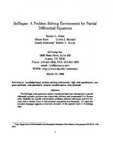
Fig. 4. Three dimensional prints generated with selective laser sintering
demonstration purposes, we have also made use of 3D-printing techniques (see Fig. 4). Two morphologies generated by the PORAG model were constructed using the selective laser sintering (SLS) technique (reviewed in Ref. [22]). Such three-dimensional prints make it possible to visually compare the simulated morphologies to real morphologies in the user’s office (tier VI). To enable more extensive comparison between real and simulated morphologies, several corals were scanned using a medical CT-scanner [5]. These morphologies were converted to a format that can be read by the iterative geometric construction library. In this way the simulated and real objects could be visualised using identical tools, and a fair visual comparison could be made: a “Turing test” [23] for models of morphogenesis. The availability of coral scans also enabled us to apply the analysis tools developed for the simulated corals on the real ones as well. A number of legacy codes for such analysis tools are available in our group, which should finally be all made available through the PSE. The dashed arrow pointing from the visualisation back to the user’s applications indicates the possibility to use the three-dimensional geometric output as the initial geometry for a new simulation. Also, it indicates the future desire for interactive simulation, where the user would be able to interact with the simulation by manipulating the visualisation. For example, the boundary conditions could be changed, to simulate changing environmental conditions. Another example could be to manipulate the position of the growing coral to simulate transplantation experiments, or to remove branches. Such interactive simulation is already applied in simulations of interactive vascular reconstructions developed in our group [24].
8
4
Discussion
In this paper we have introduced and analysed a prototypical problem solving environment for the simulation of coral morphogenesis. Such a PSE enables marine biologists to experiment with the coral growth simulation, without the need for specific technical training or knowledge about the simulation methods. Using the web front-end, the user can specify simulation parameters, an initial geometry, the growth function, and start the simulation, while the parallel system architecture remains hidden. Currently, our system is not yet able to warn the user in case he would choose combinations of parameters that are known to result in incorrect results. In future version of the PSE such knowledge will be included. For example, knowledge about the valid combinations of flow velocity and diffusion coefficients [15] would be easily included in the PSE. Although the interaction through a web-interface makes the simulation system accessible to computationally untrained scientists, it may be limiting to others. Therefore, we have constructed the PSE according to a tiered and modular architecture. The deeper one proceeds in this architecture, the more computational skills are needed with the gain of more flexibility. For example, if one is not satisfied by simulation set-ups offered by the web-server, a new set-up can be created using high level C++ objects. This requires some basic knowledge on C++ programming, but the deeper geometric library and CFD codes can be safely considered a black box. If desired, such a new simulation set-up could be interfaced to the web-server, but this is not necessarily required. With some more technical knowledge, the CFD and A-D solvers can be swapped for different solvers, thanks to the modular architecture. Indeed we are planning to do so in the near future, since we are now running into the limits of these solvers. The LBGK method we currently use is not able to simulate turbulent flows and the current A-D method produces incorrect results when advective transport becomes much more important than diffusive transport [15]. Simulations of morphogenesis generally are not only high performance applications, but also high throughput applications. In order to understand the role of each of the parameters in a model of morphogenesis, one should be able to do parameter sweeps to construct so called “morphospaces” [25]. These theoretical orderings of morphologies are used to find non-existing shapes produced by the modelled morphogenetic mechanism, and are helpful in analysing the modelled mechanism and in interpreting the functional advantage of existing morphologies. Realistic simulations of morphogenesis are computationally very expensive (a typical simulation of the PORAG model takes 18 to 36 hours on 16 processors of a 500 Mhz Pentium-3 workstation cluster). This makes such extensive parameter sweeps not yet feasible. Conventional high throughput architectures such as Condor [26] are not suitable for managing high performance applications. Conversely, architectures for dynamically managing high performance applications, such as Dynamite [27] (a Grid enabled version is currently being constructed) would allow efficient execution of the simulators in a dynamic and heterogeneous resource such as the Grid. However, Dynamite was not constructed for high throughput computing. Grid enabled parameter sweep architectures, such
9
as Nimrod/G [28] do enable this. In future work we plan to interface our morphogenesis PSE to a combination of Dynamite and Nimrod/G in order to allow for the efficient construction of morphospaces on computational grids.
5
Acknowledgements
We would like to thank Robert van Liere (CWI, Amsterdam) for visualising our simulation results on the Personal Space Station, Robert Belleman (UvA) for the visualisations on the UvA-DRIVE and CAVE systems and Leo E.H. Lampmann (St. Elisabeth Ziekenhuis, Tilburg) for making three-dimensional scans of real corals, that were kindly made available by Mark Vermeij (Cooperative Institute for Marine and Athmospheric Studies, Miami) and Rolf Bak (Netherlands Institute for Sea Research and UvA). We thank Zeger Hendrikse (UvA) and Kamil Iskra (UvA) for fruitful discussions.
References 1. Newman, S.A.: Developmental mechanisms: putting genes in their place. J. Biosci. 27 (2002) 97–104 2. Segel, L.A.: Computing an organism. PNAS 98 (2001) 3639–3640 3. Hogeweg, P.: Computing an organism: on the interface between informatic and dynamic processes. Biosystems 64 (2002) 97–109 4. Kaandorp, J.A., Lowe, C.P., Frenkel, D., Sloot, P.M.A.: Effect of nutrient diffusion and flow on coral morphology. Phys. Rev. Lett. 77 (1996) 2328–2331 5. Kaandorp, J., K¨ ubler, J., eds.: The algorithmic beauty of seaweeds, sponges and corals. The virtual laboratory. Springer, Berlin Heidelberg New York (2001) 6. Kaandorp, J.A., Sloot, P.M.A.: Morphological models of radiate accretive growth and the influence of hydrodynamics. J. Theor. Biol. 209 (2001) 257–274 7. Merks, R.M.H., Hoekstra, A.G., Kaandorp, J.A., Sloot, P.M.A.: Models of coral growth: Spontaneous branching, compactification and the Laplacian growth assumption. Accepted for publication in Journal of Theoretical Biology (2003) 8. Merks, R., Hoekstra, A., Kaandorp, J., Sloot, P.: Spontaneous branching in a polyp oriented model of stony coral growth. In Sloot, P., Tan, C.K., Dongarra, J.J., Hoekstra, A.G., eds.: International Conference on Computational Science (ICCS), Lecture Notes in Computer Science (LNCS). Volume 2329., Amsterdam, the Netherlands, Springer-Verlag, Berlin (2002) 88–96 9. Merks, R.M.H., Hoekstra, A.G., Kaandorp, J.A., Sloot, P.M.A.: Branching and morphologic plasticity in stony corals: the polyp oriented approach. Submitted (2002) 10. Gallopoulos, E., Houstis, E., Rice, J.R.: Computer as thinker/doer: Problemsolving environments for computational science. IEEE Comput. Sci. Eng. 1 (1994) 11–23 11. Rice, J.R., Boisvert, R.F.: From scientific software libraries to problem solving environments. IEEE Comput. Sci. Eng. 3 (1996) 44–53 12. Witten Jr., T., Sander, L.: Diffusion-limited aggregation, a kinetic critical phenomenon. Phys. Rev. Lett. 47 (1981) 1400–1403
10 13. Succi, S.: The Lattice Boltzmann Equation: for Fluid Dynamics and Beyond. Numerical Mathematics and Scientific Computation. Oxford University Press, Oxford New York (2001) 14. Lowe, C.P., Frenkel, D.: The super long-time decay of velocity fluctuations in a two-dimensional fluid. Physica A 220 (1995) 251–260 15. Merks, R.M.H., Hoekstra, A.G., Sloot, P.M.A.: The moment propagation method for advection-diffusion in the lattice Boltzmann method: validation and P´eclet number limits. J. Comput. Phys. 183 (2002) 563–576 16. Kandhai, D., Koponen, A., Hoekstra, A.G., Kataja, M., Timonen, J., Sloot, P.M.A.: Lattice-Boltzmann hydrodynamics on parallel systems. Comput. Phys. Commun. 111 (1998) 14–26 17. Afsarmanesh, H., Belleman, R.G., Belloum, A.S.Z., Benabdelkader, A., van den Brand, J.F.J., Eijkel, G.B., Frenkel, A., Garita, C., Groep, D.L., Heeren, R.M.A., Hendrikse, Z.W., Hertzberger, L.O., Kaandorp, J.A., Kaletas, E.C., Korkhov, V., de Laat, C.T.A.M., Sloot, P.M.A., Vasunin, D., Visser, A., Yakali, H.H.: VLAMG: A Grid-based virtual laboratory. Scientific Programming: Special Issue on Grid Computing 10 (2002) 173–181 18. Belleman, R., Stolk, B., de Vries, R.: Immersive virtual reality on commodity hardware. In Lagendijk, R., Heijnsdijk, J., Pimentel, A., Wilkinson, M., eds.: Proceedings of the 7th annual conference of the Advanced School for Computing and Imaging, Heijen, the Netherlands, Advanced School for Computing and Imaging (ASCI) (2001) 297–304 19. Mulder, J., van Liere, R.: The personal space station: Bringing interaction within reach. In: Proceedings of VRIC2002; 4th Virtual Reality International Conference, Laval, France (2002) 73–81 20. Poston, T., Serra, L.: The virtual workbench: Dextrous VR. In G. Singh, S.K.F., Thalmann, D., eds.: Proceedings of the VRST’94—Virtual Reality Software and Technology, Singapore, World Scientific (1994) 111–122 21. Cruz-Neira, C., Sandin, D., DeFanti, T.: Surround-screen projection-based virtual reality: The design and implementation of the CAVE. In: SIGGRAPH ’93 Computer Graphics Conference, ACM SIGGRAPH (1993) 135–142 22. Kruth, J., Leu, M., Nakagawa, T.: Progress in additive manufacturing and rapid prototyping. Annals of the CIRP 47 (1998) 525–540 Keynote paper. 23. Turing, A.M.: Computing machinery and intelligence. Mind: A quarterly review of psychology and philosophy 59 (1950) 433–460 24. Belleman, R., Sloot, P.: The design of dynamic exploration environments for computational steering simulations. In Bubak, M., Mo´sci´ nski, J., Noga, M., eds.: Proceedings of the SGI Users’ Conference, Krak´ ow, Poland, Academic Computer Centre CYFRONET AGH (2000) 57–74 25. McGhee, Jr., G.R.: Theoretical Morphology: The concept and its applications. Colombia University Press (1999) 26. Basney, J., Livny, M.: Deploying a high throughput computing cluster. In Buyya, R., ed.: High Performance Cluster Computing. Volume 1. Prentice Hall PTR (1999) 27. Iskra, K.A., Hendrikse, Z.W., van Albada, G.D., Overeinder, B.J., Sloot, P.M.A.: The implementation of Dynamite — an environment for migrating PVM tasks. Operating Systems Review 34 (2000) 40–55 28. Abramson, D., Giddy, J.: Scheduling large parametric modelling experiments on a distributed meta-computer. In: PCW ’97, Australian National University, Canberra (1997) P2–H–1 – P2–H–8