A Problem Solving Environment for Stochastic Biological Simulations Joseph R. Peterson∗ , Michael J. Hallock† , John A. Cole‡ , and Zaida Luthey-Schulten§ ∗
Department of Chemistry, University of Illinois at Urbana-Champaign, Urbana, Illinois 61801. Email:
[email protected] † School of Chemical Sciences, University of Illinois at Urbana-Champaign, Urbana, Illinois 61801 ‡ Department of Physics, University of Illinois at Urbana-Champaign, Urbana, Illinois 61801 § Beckman Institute, University of Illinois at Urbana-Champaign, Urbana, Illinois 61801 Email:
[email protected], Telephone: (217) 333–3518, Fax: (217) 244–3186
Abstract—Stochastic simulations of biological systems vary widely in scope from reaction modules, to single cells, to cell colonies. While the same techniques for sampling the stochastic equations governing cellular processes apply to all these systems, the setup of the simulation volume and initial state for the simulations differ significantly. Lattice Microbes is a GPU accelerated stochastic biological problem solving environment with a general interface that meets the diverse requirements of these types of biological simulations. The software includes a Python interface that allows facile customization of the simulation setup and on-the-fly modification of the simulation state with access to highly optimized, compiled algorithms for solving the stochastic equations. Here we describe the interface to Lattice Microbes and present several examples of very different simulations that were rapidly prototyped in Python. Two examples show standard stochastic biochemical problems. As an example of the true utility of the Python interface, the highly optimized method for sampling the reaction-diffusion master equation in Lattice Microbes is coupled to the COBRA toolbox, a Python package that solves a linear programming problem representing the steady-state reaction flux through the full metabolic model of the cell. This final example shows how the Python interface allows the GPU optimized code to be used to interface with other methods.
I.
[3] and how neurons relay signals from the previous to the next neuron in the chain [4]. This latter example is especially important for studies of human physiology and neurodegenerative disease. Studying the interactions between cells, such as neighboring bacteria in a colony or neighboring neurons in the brain can require several different computational approaches integrated into a multi-scale simulation setup. In this respect, the Python scripting language offers the modeler a unique environment in which to simultaneously make use of multiple different modeling libraries in an intuitive way. As more biological data becomes available, and models become more complete, computational biologists have increasingly relied on high performance computing (HPC) resources, and the use of Python in the HPC arena has grown. The focus of this article is to briefly describe several aspects of the Lattice Microbes problem solving environment—pyLM and pySTDLM—which are new Python libraries designed to facilitate use of the GPUaccelerated Lattice Microbes stochastic simulation software [2], [5]–[7], as well as to give examples of its application to problems of real scientific interest.
I NTRODUCTION
All living organisms rely on complex networks of biochemical reactions in order to extract energy from their surroundings, grow, and reproduce. These networks can contain thousands of interacting species—many in relatively small copy numbers—and can involve strong positive and negative feedback schemes that enable the organisms to tightly control their behavior. Modeling the average behavior of these types of networks is relatively straightforward by integrating, for example, coupled sets of ordinary differential equations (ODE); but understanding the unique behavior of individual cells requires explicit accounting of both the inherent randomness of all chemical processes, as well as the spatial heterogeneity within real living organisms. Numerous anomalous and bistable systems can only be modeled appropriately when stochasticity is included. The lac genetic switch, for example, exhibits a range of inducer concentrations over which random chemical events can drive individual cells growing in macroscopically identical environments into very different states of gene expression and behavior [1], [2]. Stochasticity also plays an important role in signal transduction and how cells respond to external stimuli. Examples include cell response/movement to external nutrients
A. Chemical Master Equation The probability that a simulation will be in a given state— defined as the numbers of each modeled species at a given instant—evolves in time according to the Chemical Master Equation (CME). Unlike ODE representations of a reaction network which treat concentrations as continuous and their evolution as deterministic, the CME is inherently probabilistic and species numbers are treated as discrete. The form of the CME is shown in Equation 1. Reactions are reflected by changes in the system state, ~x and the probability of a particular reaction occurring is the product of the number of particles of the reactants, ~xi ∈ ~x and their propensity to react, ar (~x, t), which is related to the macroscopic (deterministic) rate constant. By summing over all the probabilities to react backwards (the first term in the summation), and to react forward (the second term in the summation) for all reactions, the total probability of the system moving out of a given state, ~x, at the given time, t, can be calculated. Problems that invoke the CME require reactions and species to be specified, reaction rate laws and kinetic parameters, as well as any additional rules that should be applied.
R X
∂P (~x, t) = −ar (~x)P (~x, t) + ar (~x − ~sr )P (~x − ~sr , t) (1) ∂t r=1 The CME can only be solved analytically for a very few simple systems, and must be approximated via sampling techniques for most realistic systems. Several methods have been developed to sample the CME based mostly on Gillespie’s Stochastic Simulation Algorithm (SSA) [8] and extensions to the method including the τ -leaping method [9], the compositerejection method [10] and the optimized direct method [11] to name a few. For a complete review of the CME, the reader is directed to the 2007 manuscript by Gillespie [12]. Several conditions must hold for the CME to apply to a given system. The first is the “well-stirred” assumption which presupposes that the reactions occur at timescales much slower than diffusion—analogous to an ODE system. Another is that each reaction is a completely independent event, describable as a Markovian processes. To investigate scenarios that relax the first of these conditions, a spatially-resolved approach must be used. B. Reaction-Diffusion Master Equation The Reaction-Diffusion Master Equation (RDME) describes the time evolution of spatially-resolved states, and is necessary where diffusion and reaction occur on the similar enough timescales that gradients of species concentrations may arise in the system—analogous to a PDE system. In addition to a term functionally identical to the CME that describes chemical reactivity, the RDME includes a term pertaining to the diffusion of particles through a volume, as seen in the second part of Equation 2. ˆˆ ˆ
i,j,k X V ±X N X ∂P (~x, t) = CM E + −dα xα xα v~ v P ((~ v , t) ∂t v α ζ
α α α α + dα xα xα v (~ v − 1v + 1v+ζ ) × P (~ v − 1v + 1v+ζ , t) (2)
Spatially-resolved states can be sampled via a particlebased approach, where the point particles are subjected to Brownian (random) motion and react when they are close enough (with some associated probability of reaction), or via a lattice-based approach with the simulation domain discretized to a regular lattice. In this approach, particles are placed on lattice sites, and have a probability to diffuse to neighboring lattice sites and/or to react with other particles in the same site. Each lattice site is treated as well-stirred, allowing the CME to be solved on each site independently of every other site. The form of the RDME shown above is that for a latticebased code, where the summations run over all the lattice sites v ∈ V and the probability of diffusing into neighboring sites ζ for each particular particle type α ∈ N is computed. The total probability of the system to change state is then the probability of a reaction or a diffusion event occurring. Therefore, in addition to the inputs to the CME simulation, RDME methods require spatial information of the simulated
volume and diffusion data to be specified. Both the RDME and CME may be sampled by a number of code packages available free of charge on the internet. In the next section we will discuss Lattice Microbes, a particularly powerful and efficient package for sampling the CME and RDME. In subsequent sections we will demonstrate the use of Lattice Microbes as a problem solving environment. Finally, we will conclude with a comparison of the capabilities and performance of Lattice Microbes with other software packages. II.
L ATTICE M ICROBES
Lattice Microbes is a stochastic simulation software package designed from the ground up in C++ to solve the CME and RDME on graphical processing units (GPU) [6] via a highly optimized NVIDIA CUDA implementation. It uses a lattice based approach to sample the RDME as opposed to a particle-based approach, making it more amenable to GPU programming. For this reason it has demonstrated considerable speedup over similar codes on the order of 2x for CME and 300x for RDME simulations [6] on a single GPU. Further development has culminated in a multiple-GPU version that can perform with 75% ideal strong scaling on a single node to 8 GPUs or simulate larger total volume proportional to the GPU count [7]. We have measured a total code performance of 376 GFlops on a 1 million particle, 2563 lattice RDME simulation of the bimolecular reaction, A + B ←→ C, on a Quadro 4000, equivalent to 80% peak performance. The HDF5 parallel file format [13] is used by Lattice Microbes to store data and RDME trajectories. These trajectories can be visualized with a plugin to the popular Visual Molecular Dynamics (VMD) software package [14]. Additionally, other tools, such as Matlab, can read HDF5 files, and can be used for post-processing and data analysis. In addition, the program can read the standard Systems Biology Markup Language (SBML) [15] that represents reactions in a (verbose) XML format, allowing the software to facilitate many standard reaction systems published in the format. Studies that have utilized Lattice Microbes include spatially resolved gene expression simulations [2], repressor-rebinding studies [6], characterization of sub-diffusive behavior due to crowded cellular environments [5], study of the MinDE system spontaneous oscillatory behavior in cells [7], [16], and study of emergent phenotype formation in randomly generated colonies of cells [17]. What is interesting about these studies is they contain vastly different systems and the resulting problem definitions varied considerably. This variability motivated a more user-friendly approach to interfacing with the software than originally available. To facilitate facile prototyping of these and other biological problems, we have developed a Python problem solving environment on top of Lattice Microbes. A. Python Interface At its base, a Python interface wraps the C++ API of Lattice Microbes, exposing relatively low-level program functionality to Python via Simplified Wrapper and Interface Generator (SWIG) [18]. On top of SWIG, we have developed a problem solving environment (PSE) and “standard library” in Python dubbed “pyLM” and “pySTDLM” respectively, that wrap much of the low-level functions, greatly simplifying
pyLM SWIG Interface SBML/CMD Line
Lower-Level
pySTDLM
Lattice Microbes
during execution of the simulation. The Python class is given access carte blanche to the lattice state. The modified state is then used as the starting point to resume the original RDME solver. In these ways, the Python interface can be thought of as a wrapper for a highly specialized implementation of CME and RDME solvers—similarly to how LAPACK [21] is a wrapper for solving a class of linear algebra problems. Thus, Lattice Microbes is a PSE for stochastic biological systems. The following sections will demonstrate examples of different systems implemented via this PSE. III.
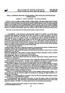
Fig. 1. A schematic showing the hierarchy of the Lattice Microbes problem solving environment (PSE). The bottom level is an optimized C++ code designed to solve various implementations the CME and RDME on GPUs. The SWIG interface implements a low-level wrapper for the C++ API of Lattice Microbes. Additionally, Lattice Microbes simulations can be defined and run from the command line tools using SBML files as definitions of the reaction network. Above this, sits the bulk of the PSE, where a high-level API implements functionality necessary to create such constructs as cells, pack them with obstacles and particles, supports time-based callbacks, and perform several post-processing functionalities. At the top level sit both a standard cell and standard reaction library of reactions, reaction systems, cell geometries, etc.
defining reaction systems, diffusion properties, cell geometries and packing of cells with objects (proteins, DNA, etc.). The hierarchy of the Lattice Microbes PSE is shown schematically in Figure 1. In addition, Lattice Microbes simulations may be initialized, launched and monitored from within a Python script or from a Python terminal. A derivable class with a callback function supports time-based interrupts that pass control and the simulation state back to the Python environment for onthe-fly modification and analysis of the system state. These facilitate, as we will demonstrate in subsequent sections, the coupling of CME or RDME with other modeling methods. Moreover, the direct access to the main lattice data structures of Lattice Microbes allows post-processing and data analysis tools to be designed within Python, allowing the use of powerful graphing libraries such as Matplotlib [19], and numerical analysis libraries NumPy and SciPy [20]. A few standard postprocessing tools that ship with pyLM are also demonstrated, especially those that link against h5py as an interface to HDF5. Mixed methods simulations rely on using multiple solvers that feed information into one another. In order to achieve this, one must be able to regularly interrupt execution of a solver in order to interrogate and manipulate its state. By allowing this to occur within a user’s Python code is a powerful feature that leverages the optimized, compiled solvers available with the flexibility and ease of use that has helped make Python so popular. A user can write very little code in order to implement what is, in actuality, a new class of solvers. Much of this is accomplished by using the advanced SWIG feature known as a director. This wraps a specialized target C++ solver class derived from the MPD-RDME solver that contains virtual methods that are called as part of the inner simulation loop. The director provides a Python class that can be targeted for inheritance as a Python solver class. The user can then override methods in the superclass that will be called
C ASE S TUDIES
Three examples of stochastic simulations prototyped in the Lattice Microbes PSE follow. CME and RDME examples are demonstrated followed by an example of more sophisticated simulation control where the RDME method has been merged with another method for biochemical simulations in an unprecedented implementation. In each case the system is described briefly, followed by identification of how the PSE facilitated the prototyping or increased legibility over the previous versions. In two cases a side-by-side comparison of the simulation specification with pyLM to the “old-way” (lowlevel API) is shown, to demonstrate how the readability of the code is enhanced. A. CME of the Two- and Thee-State Lac Genetic Switch A simple example of how noise in a biochemical process can cause cells which are initially in a similar starting state to diverge into populations with different behaviors as time progresses is the lac genetic switch in E. coli. The switch is used by the bacteria to optimize their uptake and metabolism for growth when lactose—here, called the “inducer”—is available. The scenario is shown schematically in Figure 4. Switching between the various states is a stochastic event resulting in two populations under certain inducer concentrations. Two models of the lac genetic switch have been proposed, the two-state and the three-state. The two-state switch is like a light switch, existing in on or off states. Both switches result in bimodal populations where some cells are “induced” and others are “uninduced” meaning they are expressing the lacY [2], [22], some are on and others are off, respectively. The three-state switch includes a looped state that allows even greater range of bistability int he population. Each scenario will be discussed in turn. The two-state switch, shown in Figure 3b, demonstrates the normal behavior of a cell growing in lactose the expression of the gene is either on or off. Details of the model can be found elsewhere [2]. The original code for the low-level Python interface to set up the simulation is shown in Listing 1. Specification of the input parameters for the reaction and diffusion models via the command line requires that the user manually construct tables of data, and must maintain a constantly ordered enumeration of the chemical species. This process is tedious for larger systems and is difficult to extract meaning from simply by looking at it. A superior solution that conveys not only the simulation design, but also meaning, is that of the PSE implementation (Listing 2). The first thing to
Uninduced State
Looped State
lac operon
Gene Repression
Inducer Import
DNA
LacY
mRNA
Ribosome
LacI
Unfolded LacY
Substrate Depletion
Active Transport
εkts
kunloop
ktl
kloop
Off State
Repressor Tetramer
Passive
Inducer
Transport
Inducer
Induced State
On State Operator
kon
koff Promoter
kts Operator
Gene
ktl mRNA
Free Repressor Dimer with Inducer Bound
(a) lac System Operation
kdegm kdegp
LacY Protein
Active Transport
Degraded
(b) The lac Switch Model
Fig. 3. The lac system is used to change the metabolism of an E. coli cell when the lactose nutrient is available. A schematic of the time course is shown in (a) where a the inducer finds its way into a cell and binds to the lac repressor protein, causing the protein to detach and allows transcription of the lac operon. This creates messenger RNA molecules that can then be translated by the ribosomes into proteins. One protein, LacY, transports more inducer into the cell, providing a positive feedback loop, reducing the probability of the repressor to live on the DNA, acting as a feedforward loop pushing the cell into an “induced” state. The modeled system is shown in (b) where the dotted box represents just the portions that are represented in the two-state model. The three-state system comprises all the portions of the diagram. Figures adapted from [2], [22].
notice is that the use of the “named” species. After species are defined, we use the addReaction(...) function to define a chemical reaction in the system. It can be seen that no stoichiometry or dependency data need be supplied, as these are implicit in the form of the arguments to the function. For example, it is obvious that addReaction((’R2’,’O’), product=’R2O’, rate=2.43e-6) is a 2nd order reaction that depends on species R2 and O. This example demonstrates how the Lattice Microbes PSE used the power of Python dynamic typing to cover up what is already intuitive to the scientist about the form of a particular reaction. Listing 1. Code used to set up the lac system using the traditional method calling command line utilities that interface with Google Protocol Buffers. # Define Stoichiometry matrices lm_setrm lac.lm.lm numberSpecies=14 numberReactions =23 "InitialSpeciesCounts =[9,1,0,0,0,0,0,0,0,0,30,2408,2408,0]" "ReactionTypes= [2,2,2,1,1,1,1,1,1,1,2,2,2,2,1,1,1,1,1,1,2,1,1]" "ReactionRateConstants(0:22)= [2.43e6;1.21e6;2.43e4;6.3e-4;6.3e-4;3.15e-1; 1.26e-1;4.44e-2;1.11e-2;2.1e-4;2.27e4;1.14e4;6.67e2; 3.33e2;2e-1;4e-1;1;2;2.33e-3;2.33e-3;3.03e4; 1.2e-1;1.2e1]" "StoichiometricMatrix(0:13,0:22)= [-1,0,0,1,0,0,0,0,0,0,-1,0,0,0,1,0,0,0,0,0,0,0,0; -1,-1,-1,1,1,1,0,0,0,0,0,0,0,0,0,0,0,0,0,0,0,0,0; 1,0,0,-1,0,0,0,0,0,0,0,0,-1,0,0,0,1,0,0,0,0,0,0; 0,-1,0,0,1,0,0,0,0,0,1,-1,0,0,-1,1,0,0,0,0,0,0,0; 0,1,0,0,-1,0,0,0,0,0,0,0,1,-1,0,0,-1,1,0,0,0,0,0; 0,0,-1,0,0,1,0,0,0,0,0,1,0,0,0,-1,0,0,0,0,0,0,0; 0,0,1,0,0,-1,0,0,0,0,0,0,0,1,0,0,0,-1,0,0,0,0,0; 0,0,0,0,0,0,1,0,-1,0,0,0,0,0,0,0,0,0,0,0,0,0,0; 0,0,0,0,0,0,0,1,0,-1,0,0,0,0,0,0,0,0,0,0,-1,1,1; 0,0,0,0,0,0,0,0,0,0,-1,-1,-1,-1,1,1,1,1,1,-1,0,0,1; 0,0,0,0,0,0,0,0,0,0,0,0,0,0,0,0,0,0,0,0,0,0,0; 0,0,0,0,0,0,0,0,0,0,0,0,0,0,0,0,0,0,-1,1,-1,1,0; 0,0,0,0,0,0,0,0,0,0,0,0,0,0,0,0,0,0,0,0,1,-1,-1; 0,0,0,0,0,0,0,0,1,1,0,0,0,0,0,0,0,0,0,0,0,0,0]"
"DependencyMatrix(0:13,0:22)= [1,0,0,0,0,0,0,0,0,0,1,0,0,0,0,0,0,0,0,0,0,0,0; 1,1,1,0,0,0,0,0,0,0,0,0,0,0,0,0,0,0,0,0,0,0,0; 0,0,0,1,0,0,0,0,0,0,0,0,1,0,0,0,0,0,0,0,0,0,0; 0,1,0,0,0,0,0,0,0,0,0,1,0,0,1,0,0,0,0,0,0,0,0; 0,0,0,0,1,0,0,0,0,0,0,0,0,1,0,0,1,0,0,0,0,0,0; 0,0,1,0,0,0,0,0,0,0,0,0,0,0,0,1,0,0,0,0,0,0,0; 0,0,0,0,0,1,0,0,0,0,0,0,0,0,0,0,0,1,0,0,0,0,0; 0,0,0,0,0,0,0,0,1,0,0,0,0,0,0,0,0,0,0,0,0,0,0; 0,0,0,0,0,0,0,0,0,1,0,0,0,0,0,0,0,0,0,0,1,0,0; 0,0,0,0,0,0,0,0,0,0,1,1,1,1,0,0,0,0,0,1,0,0,0; 0,0,0,0,0,0,0,0,0,0,0,0,0,0,0,0,0,0,0,0,0,0,0; 0,0,0,0,0,0,0,0,0,0,0,0,0,0,0,0,0,0,1,0,1,0,0; 0,0,0,0,0,0,0,0,0,0,0,0,0,0,0,0,0,0,0,0,0,1,0; 0,0,0,0,0,0,0,0,0,0,0,0,0,0,0,0,0,0,0,0,0,0,0]" # Set Timesteps and run simulation lm_setp lac.lm writeInterval=1e-5 maxTime=36000 lm -r 1-1 -ws -f lac.lm Listing 2. Code used to set up the lac system using the new pyLM interface. Some reactions are omitted for brevity. from pyLM import * from pyLM.units import * from pySTDLIB import * # Create our simulation object sim=CME.CMESimulation() # Add the reactants species = [’R2’,’O’,’R2O’,’IR2’,’IR2O’,’I2R2’,’I2R2O ’,’mY’,’Y’,’I’,’Iex’,’YI’] sim.defineSpecies(species) # Add the reactions # Lac operon regulation sim.addReaction(reactant=(’R2’,’O’), product=’R2O’, rate=2.43e6) sim.addReaction((’IR2’,’O’), ’IR2O’, 1.21e6) sim.addReaction((’I2R2’,’O’), ’I2R2O’, 2.43e4) sim.addReaction(’R2O’, (’R2’,’O’), 6.30e-4) sim.addReaction(’IR2O’, (’IR2’,’O’), 6.30e-4) sim.addReaction(’I2R2O’, (’I2R2’,’O’), 3.15e-1) # More reactions... ...
# Populate the model with particles # All other species start with 0 particles sim.addParticles(species=’R2’, count=9) sim.addParticles(species=’R2O’, count=1) sim.addParticles(species=’Y’, count=30) sim.addParticles(species=’I’, count=2408) sim.addParticles(species=’Iex’, count=2408)
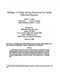
Define Simulation Instances
If RDME Simulation
Yes
Define Regions
No
# Run the simulation for 10 hours sim.run("lac2state.lm",method="lm::cme:: GillespieDSolver")
Yes
Define Geometry/ Pack Obstacles
No
Discretize to Lattice
Customize Simulation
If Custom Events
# Save the simulation state to a file sim.save("lac2state.lm") # Check that simulation parameters are valid sim.check()
Define Species/ Add Reactions
If RDME Simulation
# Set times sim.setWriteInterval(microsecond(10.0)) sim.setSimulationTime(36000.0)
Yes
Define Solver and hookSimulation()
No
Run System
Post Process Data
The three-state switch, also shown in Figure 3b, demonstrates behavior of the cell growing in an analog of lactose, where the DNA is either on, off or in a looped state. Details of the model can be found elsewhere [22]. The setup of the model is similar to Listing 2. To examine the results of the two-state switches, we turn to two functionalities of the post-processing tools of pySTDLM. A representative time trace of protein and RNA number of a cell that goes from uninduced to included is shown in Figure 4 alongside a trace for a cell that remains uninduced over the ten hour period. Only one Python command was used to plot each figure, namely plotSpeciesTrace(filename=’lac2state.lm’, species=[‘‘mY",‘‘Y"],outputFile= "uninduced.pdf", format="pdf",replicate=1). This command can be used with any number of species for any replicate sampling of the CME. This and many other plotting functions are available in the PSE, which also act as examples of how to write more complex post-processing functions that interface with HDF5. The two traces in the figure show the difference between two phenotypes, one that turns on, and one that remains off. To study how the populations change with time, we extracted the time course for each replicate and grouped them using the k-Means implementation in NumPy into two populations. The time course is shown in Figure 5. Thus, the Python interface not only allows easy post-processing using our commands, it allows coupling with all of the possible Python modules for scientific computing such as SciPy and NumPy and many others. B. RDME of the MinDE System
Fig. 2. A standard workflow used to set up a stochastic simulation with Lattice Microbes PSE. The unique customization features that really constitute the PSE are in the green and orange shaded boxes. The “Customize Simulation” step allows the user to control on a per-particle or per-lattice site basis the exact definition of the simulation volume. The definition of the solver, specifically the implementation of the hookSimulation() function allows the user to specify custom behavior and modify the simulation state at a specified time interval.
In E. coli the location of the constriction ring that squeezes the middle of the mother cell forming two daughter cells is controlled by the MinDE protein system. The system involves the interactions between the MinD and MinE protein, which form moving waves set up an oscillation of the location of the membrane bound proteins from one end of the cell to the other. This oscillation creates a relative low density of MinD at the center (perpendicular to the long dimension) of the cell, allowing another protein to bind and constrict the membrane.
250
2500
mRNA LacY
Number
2000
Number
200
mRNA LacY
150
1500
100
1000
50
500
00
4
2
6
8
Time (hr)
10
(a) Cell in the uninduced state
00
2
4
6
Time (hr)
8
10
(b) Cell in the induced state
Fig. 4. Two time courses generated by the plotSpeciesTrace(...) command discussed in the text. The plotting commands return handles of the plots to the user for customization. The plots demonstrate the behavior of two cells simulated with the same starting conditions which diverge in their behavior over time. In (a) the cell does not move into the “induced” state over the 10 hours simulated, in contrast to (b) where there is a large increase in the number of LacY transport proteins at about 4 hours which provides positive feedback to the lac switch, causing the cell to rapidly move into the induced state between 4 and 8 hours.
is added from pySTDLM which would have taken nine lines of boilerplate code in the past, is added with a single line. This process can be compared to the low-level API code which is considerably more difficult to read as demonstrated in Listings 4 and 5.
Cells per Cluster
100 80 60 40
Listing 3. Code that sets up the MinDE protein system in a capsule shaped cell 4 micrometers long with a random packing of proteins. from pyLM import * from pySTDLM import *
Induced Uninduced
# Create our simulation object sim=RdmeSimulation(dimensions=micron (1.024,1.024,4.096), spacing=nm(16))
20 00
2
4
6
Time (hr)
8
10
Fig. 5. A time course pulled out by clustering the cells based on the number of LacY protein, which were initially in the same state, into two populations. It can be seen that onset of induction occurs around 4 hours. By the end of the simulation one third of the cells have become induced. A similar analysis of mRNA number shows no trend, suggesting that experiments that measure the mRNA number alone will not be able to distinguish the phenotype of a cell.
The system is diagramed in Figure 6a, and shows how MinE interacts with MinD to expel it from the membrane, allowing MinD to then diffuse through the cytosol and rebind to the membrane at the front of the traveling wave. The pyLM code necessary to set up this simulation is shown in Listing 3. Several useful features of pyLM can be seen in the code. The first is the automatic unit conversion accomplished by the micron() and nm() functions which increase the readability. Also, the use of the addMinDESystem() from the pySTDLM decreases the amount of code required to set up this standard stochastic reaction system which is similar in style to that shown in the CME simulation above. In addition to a standard cell geometry
# Build a capsid cell sim.buildCapsidCell(length=micron(4), diameter= micron(1), membraneThickness=nm(32)) # Add the MinDE system from pySTDLM addMinDESystem(sim) # Populate the model with particles sim.addParticles(species=’minDatp’, region=’ cytoplasm’, count=1758) sim.addParticles(’minDadp’, ’cytoplasm’, 1758) sim.addParticles(’minE’, ’cytoplasm’, 914) # Set times sim.setWriteInterval(ms(10.0)) sim.setLatticeWriteIntervale(ms(10.0)) sim.setTimestep(microseconds(50.0)) sim.setSimulationTime(900.0) # Run Simulation sim.save("MinDE.lm") sim.run("MinDE.lm",method="lm::rdme::MpdRdmeSolver") Listing 4. Code in the previous Lattice Microbes version to set up the MinDE system. # Create the simulation file. lm_sbml_import MinDE.lm min_division.sbml lm_setdm ecoli.lm PlaceParticles=False numberReactions=5 numberSpecies=5 numberSiteTypes=3 "latticeSize=[64,64,256]"
Cell Pole
0.1
1.5
0.09 0.08
1
0.07 0.5
0.06
Cell Center
0
0.05 0.04
-0.5
0.03
-1
Listing 5. The build_ecoli.py script used in the Listing 4. import sys import os xlen=1024e-9; ylen=1024e-9; zlen=4096e-9 cellLength=4e-6; cellRadius=500e-9; membraneThickness=32e-9 builder=LatticeBuilder(xlen,ylen,zlen,16e-9,1,0) extraCellularType=0 extraCellular=Cuboid(point(0.0,0.0,0.0), point(xlen, ylen,zlen), extraCellularType) builder.addRegion(extraCellular) membraneType=2 membrane=CapsuleShell(point(xlen/2.0,ylen/2.0,((zlen -cellLength)/2)+cellRadius), point(xlen/2.0,ylen /2.0,((zlen-cellLength)/2)+cellLength-cellRadius ), cellRadius-membraneThickness, cellRadius, membraneType) builder.addRegion(membrane) cytoplasmType=1 cytoplasm=Capsule(point(xlen/2.0,ylen/2.0,((zlencellLength)/2)+cellRadius), point(xlen/2.0,ylen /2.0,((zlen-cellLength)/2)+cellLength-cellRadius ), cellRadius-membraneThickness, cytoplasmType) builder.addRegion(cytoplasm) # Add the particles. builder.addParticles(0, 1, 1758); builder.addParticles(1, 1, 1758); builder.addParticles(3, 1, 914); # Open the file. sim=SimulationFile(sys.argv[1]) spatialModel=SpatialModel() builder.getSpatialModel(spatialModel) sim.setSpatialModel(spatialModel) # Discretize the lattice. diffusionModel=DiffusionModel() sim.getDiffusionModel(diffusionModel) lattice = ByteLattice(diffusionModel.lattice_x_size (), diffusionModel.lattice_y_size(), diffusionModel.lattice_z_size(), diffusionModel. lattice_spacing(), diffusionModel. particles_per_site()) builder.discretizeTo(lattice, 0, 0.0) sim.setDiffusionModel(diffusionModel) sim.setDiffusionModelLattice(diffusionModel,lattice) sim.close()
In the original incarnation of the MinDE simulation, the user would have to set up the lattice as well as the number of reactions, reaction rates, diffusion rates and lattice regions from bash using several utilities. The user would then use the Python interface to specify cell geometries, add particles, discretize the obstacles to a lattice. Then the user would have to actually run
MinDm occupancy (particles per site)
# Run a simulation using MPDRDME. lm_setp MinDE.lm timestep=5e-5 latticeWriteInterval =1e-2 writeInterval=1e-2 maxTime=900.0 lm -f MinDE.lm -r 1 -sl lm::rdme::MpdRdmeSolver -cr 1 -gr 1
2
Cell Axis Position (µm)
latticeSpacing=16e-9 particlesPerSite=8 " ReactionLocationMatrix(0,1:2)=[1]" " ReactionLocationMatrix(1:4,2)=[1]" " DiffusionMatrix(1:2,1:2,0:1)=[2.5e-12]" " DiffusionMatrix(2,2,2)=[1e-14]" "DiffusionMatrix (1:2,1:2,3)=[2.5e-12]" "DiffusionMatrix(2,2,4) =[1e-14]"; lm_python -s build_ecoli.py -sa MinDE.lm
0.02 -1.5
-2
0.01 6
Cell Pole 6.2
6.4
6.6
6.8 7 7.2 7.4 Simulation time (minutes)
7.6
7.8
8
0
Fig. 7. Results of the MinDE simulation for a cell 4 micrometers long—about the size of an E. coli cell just before division into two daughter cells—showing an occupancy (number of molecules bound at a given z slice) along the cell length over time. As shown, there is a low density of the MinD protein in the center of the cell around z = 0. As opposed to non-crowded models, the oscillation frequency is about 2x slower than the original model, in accordance with the one minute oscillations for a dividing cell found in experiments [23].
the simulation. Required parameters for function calls, such as builder.discretizeTo() are redundant as the user has already specified the lattice size elsewhere. Furthermore, the operation should be implicit and run just before the simulation begins. Finally, pyLM reduces the complexity of setting up a simulation by merging the several processes such as terminal commands and Python script execution to just Python script execution. C. LatticeFBA: Integrating Different Modeling Techniques Perhaps the most powerful feature of the Python interface is its capacity for rapid integration of the Lattice Microbes algorithms with other biological modeling methods [17]. Recent extensions of the Lattice Microbes software have enabled simulations to be spread across multiple GPUs [7], and an MPI version currently under development will allow simulations to be spread even further across the large numbers of CPUs and GPUs available in modern HPC machines. These advancements are making possible detailed simulations of volumes many times larger than a single cell. By simulating multiple cells simultaneously, it is possible to investigate how dense populations can give rise to local microenvironments within bacterial colonies, and how these microenvironments can affect the behavior of individual cells. Flux balance analysis (FBA) [24], [25]—which treats the metabolism of a cell as a linear programming problem and attempts to optimize the cell’s growth rate given the available nutrients—can be performed in Python using the freely available COBRApy package [26]. The development of FBA and other genome-scale models remains an active area of research involving both biological and computational scientists [27]–[30]. By integrating FBA with the Lattice Microbes problem solving environment, multiple cells can be simulated simultaneously, with each performing its own unique metabolism in response to the nutrients diffusing
Cytoplasm
MinDADP k1
k5
MinDEm
MinDATP
MinE
k4
k2
MinDm
k3
MinDm MinDm
Extracellular Space (a) MinDE System
(b) Crowded Cell
Fig. 6. The MinDE protein system (a) causes membrane bound waves that oscillate from one end of the cell to the other by subsequent binding, modification and unbinding of the MinD protein to the cell membrane. While in the cytoplasm, MinD is phosphorylated which allows it to bind to the lipid membrane, or dimerize with other MinD on the membrane. Another protein known as MinE comes in and binds to membrane bound MinE, dephosphorylating it and destabilizing its membrane interaction expelling it from the membrane. An visualization of an initial configuration with VMD [14] (b) shows the (left) crowding of the membrane by non-MinDE proteins, (center) the membrane with holes showing membrane bound positions, and (right) initial random distribution of MinD proteins on the membrane and in the cytoplasm generated by standard methods in pyLM and pySTDLM.
in the media immediately surrounding the cell. In this way, we can extend our understanding of how cells vary behaviorally to include spatial effects and the presence of neighboring cells. The methodological merger of the RDME with FBA is described in Algorithm 1. The methodological synthesis is accomplished using the director functionality of SWIG. The MPD-RDME solver in Lattice Microbes is subclassed in Python as the “FBASolver”. The class has a virtual function that is implemented in Python and performs the FBA calculation and updates the lattice before running the next RDME steps. A snippet of the code is demonstrated in Listing 6. We have applied the hybrid FBA/RDME methodology to a colony of E. coli cells. The method is fairly straightforward. Nutrients—in this case glucose and oxygen—diffuse from a constant concentration boundary outside a cluster of randomly placed cells (see Figure 8a). The diffusion is performed stochastically on a lattice (with 24 nm resolution to ensure that the entire 12.3 µm3 lattice would fit within the available device memory). After 10 µs of diffusion time (chosen to be on the order of the time required for the fastest diffusing species to traverse a cell), the simulation is paused, and an FBA step is performed for each of the 100 cells in the simulation. The particles that have diffused or been transported into each cell are counted and used to compute the time-averaged uptake rate of each nutrient for that cell. These uptake rates are used to set the appropriate upper bounds on the cell’s exchange reactions, and FBA is used to compute the flux through every reaction in the cell’s metabolic network (the Core E. coli metabolic model [31] was used; it involves on the order of 100 reactions). The results of the FBA simulations are then used to update the spatial lattice; nutrients calculated to be used by a cell are removed from the cell’s interior while byproducts predicted to
be produced by the cell are added (in both cases rounded to the nearest whole particle). The diffusion simulation is then allowed to commence, and the cycle repeats. A simple result that arose via this simulation is demonstrated in Figure 9. Listing 6. Python code that subclasses the MPD-RDME algorithm and provides time-based control of the simulation state in Python. # Define a class that performs FBA calculation class FBASolver(lm.MpdHybridSolver): # Main callback function def hookSimulation(self, lattice): print "\nFBA Step\n" for site in lattice: # Enumerate Glucose/Oxygen atoms # Run FBA Step for site in lattice: #Remove consumed particles return 1 # specify the lattice state changed
IV.
C ONCLUSION
Herein, we described a problem solving environment for biological simulations that display stochasticity. The method of approach to solving biological simulations differs significantly from other software systems designed to solve these problems. This study would not be complete however, without a comparison to other software packages that perform spatially-resolved, stochastic simulations of biochemical processes. A. Comparison to Other Stochastic Biochemical Platforms 1) Particle-Based: Smoldyn [32] uses a terse, text-based input file specification, though benefits from GPU acceleration [33], [34], which affords it 150-250x speedup, for between 300K and 3M particles (with a total of 16M particles per
a.
b.
3000 0.8 2500
0.7 0.6
2000
0.5 1500
0.4 0.3
1000
Growth rate (hr−1)
Data: Substrate concentrations on the boundary, diffusion rates, metabolic model Result: Metabolic flux trajectories, spatial simulation trajectory Initialization: Randomly place cells and discretize to lattice, import metabolic model; while t < maxT do Perform diffusion simulation of duration ∆t in Lattice Microbes; for cell ∈ Colony do for substrate ∈ SimulatedSubstrates do availableParticles ← # of substrate particles that diffused into the cell during ∆t; Upper bound on substrate exchange reaction ← availableParticles / ∆t; end Use parsimonious flux balance analysis to predict reaction flux through the constrained metabolic model; for substrate ∈ SimulatedSubstrates do particleFlux ← substrate exchange reaction flux × ∆t; if particleFlux is into the cell then Randomly remove particleFlux particles from the lattice sites inside the cell; else Randomly add particleFlux particles to the lattice sites on the periphery of the cell; end end t ← t + ∆t; end end Algorithm 1: Pseudocode describing the simulation of a colony of cells in a solution of substrates.
Acetate / Growth Rate (mmol gDwt−1)
Fig. 8. The set up of a colony simulation; (a) rod-shaped E. coli (yellow) are randomly placed in a large simulation volume. Glucose transporter enzymes (blue) are visible on the surface of each cell. (b) A slice through the colony after running for 0.1 seconds shows glucose (grey) and oxygen (red) depleted near the center of the colony. Simulations are carried out using a new implementation of the LatticeFBA method with pyLM [17].
0.2 500 0.1 0 3
4
5
6
7
8
Radius (µm) Fig. 9. Anaerobic cells at the center of a colony tend to secrete more acetate over their lifetime than do aerobic cells near the edge of the colony. This result could only be predicted by taking into account spatial heterogeneity of the system in conjunction with a full metabolic model, meaning that the unprecedented merger of RDME and FBA is a powerful new tool.
GPU), over serial CPU, code similar in magnitude to Lattice Microbes. It is a particle-based method including crowding effects via a more complex excluded volume method and thus is slower for spatial Gillespie simulations (compare 47s vs 24s for Lattice Microbes with similar accuracy) for a benchmark outlined in the Smoldyn 2.1 paper [32]. In addition, it contains a “ports” interface that allows integration to other simulation software such as VCell [35], as well as over fifty run-time commands that allow system manipulation and observation [32]. However, there is a lack of general user programability. MCell is perhaps the most mature particle-based code [36], however it trails behind Smoldyn by a factor of 2.5x performance-wise due to less efficient algorithms [33]. Simi-
larly to Smoldyn, it uses a text based input file but does not contain any additional functionality for general user-defined controls. However, out of the box, it supports many functions Lattice Microbes does not. ChemCell is written in C++ and supports parallel simulations up to 512 processors with 80% ideal scaling for simulations with 4M particles [37]. The pre- and post-processing are performed by another tool, written in Python, called Pizza.py that allows cells to be defined as meshes, includes plotting functionality via Matlab and GnuPlot and couples to VMD [14]. The pre-processing functionality of Pizza.py is most closely related to the SWIG interface to Lattice Microbes constituting primarly low-level interface. CDS [38] is perhaps the particle-based code that is closest to being a problem solving environment. Written in Java, the software contains a graphical system builder and a 3D visualization environment for watching the simulation trajectory. In addition, the module-based interface and the user defined events/actions allows customization of the method to develop specialized simulations. The event-driven paradigm allows more accurate simulation than the other particle-based simulators. The downfall of CDS is also the event-based nature which limits the timescales (order of seconds) obtainable and contains very strong dependence of the scaling on the simulation complexity (i.e. particle number, event-frequency, etc.). GridCell [39] is a novel particle-based simulator that uses a discretized spatial representation (Lattice-Boltzmann method) to speed up the performance over traditional particle-based methods. It supports SBML as well as a graphical user interface and XML definition of of input files. Some drawbacks are that it only runs on the Windows operating system and has limited user extensibility; only the simulation geometry and particle number user configurable. In addition, comparing single core benchmarks of GridCell [39] shows that it is at least an order of magnitude slower, and in some cases two orders of magnitude slower than Lattice Microbes as the number of particles becomes high. 2) Lattice-Based: MesoRD [40] is Lattice-based code that implements the Next Subvolume Method (NSM) [41], supports mean-field simulations and is generally a high-resolution modeler for stochastic RDME simulations. In the past, we have shown that Lattice Microbes is as much as 360x faster for RDME simulations using the MPD-RDME algorithm and implements the NSM is about 10x faster than in MesoRD for a characteristic simulation [6]. GMP is perhaps the closest to Lattice Microbes in algorithm design [42]. In addition, a GPU version of the code (called GPGMP) was developed that had similar performance but about 2x slower [43]. The GPGMP, however, is a 2D code, and therefore can take advantage of better memory locality than Lattice Microbes. The simulator has been applied to some interesting systems including stochastic cell migration via a hybrid RDME/Drift method that allows cells to drift through the environment [44], demonstrating their RDME implementation can be merged with other methods. However the interface is in the C++ language as opposed to the Python interface we have developed necessitating recompilation between implementations. For this reason, we believe Lattice
Microbes is a superior problem solving environment. E-Cell [45] is one more notable lattice-based method for cell simulation. It contains many deterministic and stochastic methods for solving biochemical models. In addition, it contains a rather robust, albeit low-level, Python interface that allows simulation setup, interactive modification of the simulation, and post-processing. Very little performance data is available for E-Cell so a complete comparison is not possible. B. Final Word As we showed, three examples of very different simulations were prototyped using the Python interface rather easily and legibly. Not only were traditional CME and RDME simulations set up with few lines of code, a merger of very different methods was demonstrated. The results were demonstrated via several post-processing tools included in the PSE, useful for plotting or other data analysis. Underlying all of the features is a powerful Python PSE. Python proved to be the best solution for many reasons when considering how to develop the PSE. These include fast prototyping, dynamic typing, command line interface and numerous scientific libraries available in the language. Above all, the syntactic sugar inherent to Python allows intuitive formulation of a problem, as demonstrated by the use of tuples when defining reactions. The speed of the CME/RDME implementations in conjunction with the ease of use of the Python interface shows the utility of Lattice Microbes in solving stochastic simulations. Lattice Microbes, along with user guides and example files, may be downloaded from: http://www.scs.uiuc.edu/schulten/lm. ACKNOWLEDGMENT We would like to extend our gratitude to Elijah Roberts as the original author of Lattice Microbes and for the original SWIG interface. We would like to also thank John E. Stone for his valuable insight throughout the development process. We would like to thank the NSF for grants PHY-0822613 and the DOE under grant DE-FG02-10ER6510 for funding. JRP would like to thank NIH for support under Molecular Biophysics Training Grant PHS 5 T32 GM008276. This research used resources of the Oak Ridge Leadership Computing Facility located in the Oak Ridge National Laboratory, which is supported by the Office of Science of the Department of Energy under Contract DE-AC05-00OR22725. This work used the Extreme Science and Engineering Discovery Environment (XSEDE) under charge number TG-MCA03S027, which is supported by National Science Foundation grant number OCI1053575. R EFERENCES [1]
P. J. Choi, L. Cai, K. Frieda, and X. S. Xie, “A stochastic singlemolecule event triggers phenotype switching of a bacterial cell,” Science, vol. 322, no. 5900, pp. 442–446, 2008. [2] E. Roberts, A. Magis, J. O. Ortiz, W. Baumeister, and Z. LutheySchulten, “Noise contributions in an inducible genetic switch: A wholecell simulation study,” PLoS Comput. Biol., vol. 7, no. 3, p. e1002010, Mar 2011. [3] T. S. Shimizu, S. V. Aksenov, and D. Bray, “A spatially extended stochastic model of the bacterial chemotaxis signaling pathway,” J. of Mol. Bio., vol. 329, no. 2, pp. 291–309, 2003.
[4] [5]
[6]
[7]
[8] [9]
[10]
[11]
[12] [13] [14] [15] [16] [17]
[18]
[19] [20] [21]
[22]
[23] [24]
[25]
[26]
[27]
W. Maass and A. M. Zador, “Dynamic stochastic synapses as computational units,” Neural Computation, vol. 11, no. 4, pp. 903–917, 1999. E. Roberts, J. E. Stone, L. Sepulveda, W.-M. W. Hwu, and Z. LutheySchulten, “Long time-scale simulations of in vivo diffusion using GPU hardware,” The Eighth IEEE International Workshop on HighPerformance Computational Biology, May 2009. E. Roberts, J. E. Stone, and Z. Luthey-Schulten, “Lattice microbes: high-performace stochastic simulation method for the reaction-diffusion master equation,” J. Comput. Chem., vol. 3, pp. 245–255, 2013. M. J. Hallock, J. E. Stone, E. Roberts, C. Fry, and Z. Luthey-Schulten, “Long time-scale simulations of in vivo reaction diffusion processes on multiple GPUs,” 2013, submitted. D. Gillespie, “Exact Stochastic Simulation of Coupled Chemical Reactions,” J. Phys. Chem., vol. 81, no. 25, pp. 2340–2361, 1977. M. Rathinam, L. Petzold, Y. Cao, and D. Gillespie, “Stiffness in stochastic chemically reacting systems: The implicit tau-leaping method,” J. Chem. Phys., vol. 19, no. 24, pp. 12 784–12 794, 2003. A. Slepoy, A. Thompson, and S. Plimpton, “A constant-time kinetic Monte Carlo algorithm for simulation of large biochemical reaction networks,” J. Chem. Phys., vol. 128, no. 20, p. 205101, 2008. Y. Cao, H. Li, and L. Petzold, “Efficient formulation of the stochastic simulation algorithm for chemically reacting systems,” J. Chem. Phys., vol. 121, no. 9, pp. 4059–4067, 2004. D. Gillespie, “Stochastic simulation of chemical kinetics,” Annu. Rev. Phys. Chem., vol. 58, pp. 35–55, 2007. TheHDFGroup, “Hierarchical data format version 5,” 2005–2010. [Online]. Available: http://www.hdfgroup.org/HDF5 W. Humphrey, A. Dalke, and K. Schulten, “VMD: Visual Molecular Dynamics,” J. Molec. Graphics, vol. 14, no. 1, pp. 33–38, 1996. B. Bornstein, S. Keating, A. Jouraku, and M. Hucka, “LibSBML: An API Library for SBML,” Bioinform., vol. 24, no. 6, pp. 880–881, 2008. M. Hartmann, “Stochastic Simulation of Reaction-Diffusion Systems,” Master’s thesis, Ludwig-Maximilians-Universitat Munchen, 2013. J. Cole, M. Hallock, P. Labhsetwar, J. Peterson, J. Stone, and Z. LutheySchulten, Stochastic Simulations of Cellular Processes: From single cells to colonies. Academic Press, 2013, ch. 13. D. M. Beazley, “SWIG: an easy to use tool for integrating scripting languages with C and C++,” in TCLTK’96 Proceedings of the 4th conference on USENIX Tcl/Tk Workshop, vol. 4, 1996, p. 15. J. D. Hunter, “Matplotlib: A 2D graphics environment,” Computing In Science & Engineering, vol. 9, no. 3, pp. 90–95, 2007. E. Jones, T. Oliphant, P. Peterson et al., “SciPy: Open source scientific tools for Python,” 2001–. [Online]. Available: http://www.scipy.org/ E. Anderson, Z. Bai, C. Bischof, S. Blackford, J. Demmel, J. Dongarra, J. Du Croz, A. Greenbaum, S. Hammarling, A. McKenney, and D. Sorensen, LAPACK Users’ Guide, 3rd ed. Philadelphia, PA: Society for Industrial and Applied Mathematics, 1999. T. Earnest, E. Roberts, M. Assaf, K. Dahmen, and Z. Luthey-Schulten, “DNA looping increases range of bistability in a stochastic model of the lac genetic switch,” Phys. Biol., vol. 10, 2013. D. Fange and J. Elf, “Noise-Induced Min Phenotypes in E. coli,” PLoS Comput. Biol., vol. 2, no. 6, p. e80, 2006. J. Schellenberger, R. Que, R. M. T. Fleming, I. Thiele, J. D. Orth, A. M. Feist, D. C. Zielinski, A. Bordbar, N. E. Lewis, S. Rahmanian, J. Kang, D. R. Hyduke, and B. O. Palsson, “Quantitative prediction of cellular metabolism with constraint-based models: the COBRA Toolbox v2.0,” Nat. Protoc., vol. 6, no. 9, pp. 1290–1307, 2011. N. Lewis, H. Nagarajan, and B. O. Palsson, “Constraining the metabolic genotype-phenotype relationship using a phylogeny of in silico methods.” Nat. Rev. Microbiol., vol. 10, no. 4, pp. 291–305, 2012. [Online]. Available: http://dx.doi.org/10.1038/nrmicro2737 A. Ebrahim, J. A. Lerman, B. O. Palsson, and D. R. Hyduke, “COBRApy: Constraints-Based Reconstruction and Analysis for Python,” BMC Sys. Bio., vol. 7, no. 1, 2013. J. Schellenberger, J. O. Park, T. M. Conrad, and B. Ø. Palsson, “BiGG: a Biochemical Genetic and Genomic knowledgebase of large scale metabolic reconstructions,” BMC Bioinform., vol. 11, no. 1, p. 213, 2010.
[28] [29]
[30]
[31]
[32]
[33]
[34]
[35]
[36]
[37]
[38]
[39]
[40] [41]
[42]
[43]
[44]
[45]
M. Kanehisa and S. Goto, “KEGG: kyoto encyclopedia of genes and genomes,” Nucleic Acids Research, vol. 28, no. 1, pp. 27–30, 2000. F. B¨uchel, N. Rodriguez, N. Swainston, C. Wrzodek, T. Czauderna, R. Keller, F. Mittag, M. Schubert, M. Glont, M. Golebiewski et al., “Large-scale generation of computational models from biochemical pathway maps,” arXiv preprint arXiv:1307.7005, 2013. A. Arkin, T. Brettin, D. Chivian, B. Cottingham, B. Davison, and D. Paramvir, “DOE Systems Biology Knowledgebase,” Sep. 2013. [Online]. Available: http://kbase.science.energy.gov/ J. Orth, R. Fleming, and B. Palsson, “10.2.1-Reconstruction and use of microbial metabolic networks: the core Escherichia coli metabolic model as an educational guide,” EcoSal-Escherichia coli and Salmonella Cellular and Molecular Biology, 2010. S. Andrews, N. Addy, R. Brent, and A. Arkin, “Detailed Simulations of Cell Biology with Smoldyn 2.1,” PLoS Comput. Biol., vol. 6, no. 3, p. e1000705, 2010. D. Gladkov, S. Alberts, R. D’Souza, and S. Andrews, “Accelerating the Smoldyn Spatial Stochastic Biochemical Reaction Network Simulator Using GPUs,” in HPC’11 Proceedings of the 19th High Performance Computing Symposia, 2011, pp. 151–158. L. Dematte´e, “Parallel particle-based reaction diffusion: a GPU implementation,” in Ninth International Workshop on Parallel and Distributed Methods in Verification/Second International Workshop on High Performance Computational Systems Biology, 2010, pp. 67–77. I. Moraru, J. Schaff, B. Slepchenko, M. Blinov, F. Morgan, A. Lakshminarayana, F. Gao, Y. Li, and L. Loew, “Virtual Cell modeling and simulation software environment,” IET Syst. Biol., vol. 2, no. 5, pp. 352–362, 2008. J. Stiles, D. van Helden, T. B. Jr., E. Salpeter, and M. Saltpeter, “Miniature endplate current rise times < 100 µs from improved dual recordings can be modeled with passive acetylcholine diffusion from a synaptic vesicle,” PNAS, vol. 93, no. 12, pp. 5747–5752, 1996. S. Plimpton and A. Slepoy, “Microbial Cell Modeling via Reactive Diffusive Particles,” J. of Phys.: Conference Series, no. 16, pp. 305– 309, 2005. M. Byrne, M. Waxham, and Y. Kubota, “Cellular Dynamics Simulator: An Event Driven Molecular Simulation Environment for Cellular Physiology,” Neuroinform., vol. 8, no. 2, pp. 63–82, 2010. L. Boulianne, S. A. Assaad, M. Dumontier, and W. Gross, “GridCell: a stochastic particle-based biological system simulator,” BMC Sys. Bio., vol. 2, no. 66, 2008. J. Hattne, D. Fange, and J. Elf, “Stochastic reaction-diffusion simulation with MesoRD,” Bioinform., vol. 12, no. 21, pp. 2923–2924, 2005. J. Elf and M. Ehrenberg, “Spontaneous separation of bi-stable biochemical systems into spatial domains of opposite phases,” Syst. Biol., vol. 2, no. 1, pp. 230–236, 2004. J. Rodr´ıguez, J. Kaandorp, M. Dobrzy´nski, and J. Blom, “Spatial stochastic modeling of the phosphenolpyruvate-dependent phosphotransferase (PTS) pathway in Escherichia coli,” Bioinform., vol. 22, no. 15, pp. 1895–1901, 2006. M. Vigelius, A. Lane, and B. Meyer, “Accelerating Reaction-Diffusion Simulations with General-Purpose Graphics Processing Units,” Bioinform., vol. 27, no. 2, pp. 288–90, 2011. M. Vigelius and B. Meyer, “Multi-Dimensional, Mesoscopic Monte Carlo Simulations of Inhomogeneous Reaction-Drift-Diffusion Systems on Graphics-Processing Units,” PLoS One, vol. 7, no. 4, p. e33384, 2012. N. Ishii, M. Robert, Y. Nakayama, A. Kanai, and M. Tomita, “Toward large-scale modeling of the microbial cell for computer simulations,” J. Biotech., vol. 113, pp. 281–294, 2004.