VIZCRAFT: A Problem Solving Environment for Configuration Design ...

MAD Center VIZCRAFT: A PROBLEM SOLVING ENVIRONMENT FOR CONFIGURATION DESIGN OF A HIGH SPEED CIVIL TRANSPORT

A. Goel, C.A. Baker, C.A. Shaffer, B. Grossman W.H. Mason, L.T. Watson and R.T. Haftka

MAD Center Report 99-06-01

Multidisciplinary Analysis and Design Center for Advanced Vehicles

VIRGINIA POLYTECHNIC INSTITUTE AND STATE UNIVERSITY

Blacksburg, Virginia 24061-0203

VizCraft: A Problem Solving Environment for Configuration Design of a High Speed Civil Transport A. Goel† , C.A. Baker§, C.A. Shaffer† , B. Grossman§ , W.H. Mason§ , L.T. Watson†§ † Department of Computer Science, § Multidisciplinary Analysis and Design Center for Advanced Vehicles, Virginia Polytechnic Institute and State University, Blacksburg VA 24061 R.T. Haftka Department of Aerospace Engineering, Mechanics and Engineering Science, University of Florida, Gainesville FL 32611 Version #1, June 11, 1999 Abstract. We describe a problem solving environment named VizCraft that aids aircraft designers during the conceptual design stage. At this stage, an aircraft design is defined by a vector of 10–30 parameters. The goal is to find a vector that minimizes a performance-based objective function while meeting a series of constraints. VizCraft integrates simulation code to evaluate a design with visualizations for analyzing a design individually or in contrast to other designs. VizCraft allows the designer to easily switch between the view of a design in the form of a parameter set, and a visualization of the corresponding aircraft geometry. The user can easily see which, if any, constraints are violated. VizCraft also allows the user to view a database of designs using parallel coordinates. Keywords. Problem solving environment, multidimensional visualization, aircraft design, multidisciplinary design optimization.

1

Introduction

There is general agreement that visualization has an important role in computational science and engineering, allowing scientists to gain an understanding of their data that was not previously possible. However, lack of integration among the various software modules often separates the visualization process from the computation that generates the data. VizCraft is a design tool for the

conceptual phase of aircraft design whose goal is to provide an environment in which visualization and computation are combined. The designer is encouraged to think in terms of the overall task of solving a problem, not simply using the visualization to view the results of the computation [1]. In this paper, we describe VizCraft, a PSE that serves two purposes: (1) It provides a graphical user interface for the configuration design of a High Speed Civil Transport (HSCT) [2], and (2) It provides components for visualizing the results of the computation. The philosophy of such computing environments, and a detailed description of the working of our visualization tool are discussed. A problem solving environment (PSE) is a system that provides a complete, usable, and integrated set of high level facilities for solving problems from a prescribed domain [3]. PSEs allow users to define and modify problems, choose solution strategies, interact with and manage appropriate hardware and software resources, visualize and analyze results, and record and coordinate extended problem solving tasks. In complex problem domains, a PSE may provide intelligent and expert assistance in selecting solution strategies, e.g., algorithms, software components, hardware resources, data, etc. Perhaps most significantly, users communicate with a PSE in the language of the problem, not in the language of a particular operating system, programming lan-

VizCraft: A PSE for Configuration Design of a High Speed Civil Transport, Version #1, June 11, 1999

guage, or network protocol. Expert knowledge of the underlying hardware or software is not required. In the past, a number of PSEs for MDO applications have been developed that provide frameworks for integrating analysis codes with optimization methods in a flexible manner, besides providing GUIs for reviewing the results of an optimization process. Framework for Inter-Disciplinary Optimization (FIDO) [4] demonstrates distributed and parallel execution of MDO applications using HSCT as its example. Increasingly complex models of the HSCT have been implemented in FIDO. Besides optimization capabilities, FIDO lets the user modify input parameters while the application is executing. iSIGHT [5] provides a generic shell environment for supporting multidisciplinary optimization. A key feature of iSIGHT is its ability to combine numeric, exploratory, and heuristic methods during optimization. iSIGHT has been used to implement an HSCT application as well. The DAKOTA iterator toolkit [6] provides a flexible and extensible PSE for a variety of optimization methods including genetic algorithms. Besides optimization, methods are included for uncertainty quantification, parameter estimation, and sensitivity analysis. Messac et al. [7] describe PhysPro, a MATLABbased application for visualizing the optimization process in real time using the physical programming paradigm. Among other visualization techniques, they use parallel coordinates to visualize the design metrics of the optimization process. The Visual Computing Environment (VCE) [8] provides a coupling between various flow analysis codes involved in multidisciplinary analysis at several levels of fidelity. Kingsley et al. [9] describe Multi-Disciplinary Computing Environment (MDICE), another PSE that provides users with a visual representation of the simulations being performed. It provides a distributed, objectoriented environment where many computer programs operate concurrently and cooperatively to solve a set of engineering problems.

2

HSCT Design Problem

The HSCT design problem is to minimize the take-off gross weight (TOGW) for a 250 passenger HSCT with a range of 5, 500 nautical miles and a cruise speed of Mach 2.4. The simpli-

No. 1 2 3 4 5 6 7 8 9 10 11 12 13 14 15 16 17 18 19 20 21 22 23 24 25 26 27 28 29

Value 181.48 155.9 49.2 181.6 64.2 169.5 7.00 75.9 0.40 3.69 2.58 2.16 1.80 2.20 1.06 12.20 3.50 132.46 5.34 248.67 4.67 26.23 32.39 697.9 713.0 39000 322617 64794 33.90

2

Description wing root chord, f t leading edge break point, x f t leading edge break point, y f t trailing edge break point, x f t trailing edge break point, y f t leading edge wing tip, x f t wing tip chord, f t wing semi-span, f t chordwise location of maximum thickness leading edge radius parameter airfoil t/c ratio at wing root, % airfoil t/c ratio at leading edge break, % airfoil t/c ratio at wing tip, % fuselage axial restraint #1, f t fuselage radius at axial restraint #1, f t fuselage axial restraint #2, f t fuselage radius at axial restraint #2, f t fuselage axial restraint #3, f t fuselage radius at axial restraint #3, f t fuselage axial restraint #4, f t fuselage radius at axial restraint #4, f t location of inboard nacelle, f t location of outboard nacelle, f t vertical tail area, f t2 horizontal tail area, f t2 thrust per engine, lb mission fuel weight, lb starting cruise/climb altitude, f t supersonic cruise/climb rate, f t/min

Table 1. Twenty-nine HSCT variables and their typical values.

fied mission profile includes takeoff, supersonic cruise, and landing. A suite of low fidelity and medium fidelity analysis methods have been developed, which include several software packages obtained from NASA along with in-house software. A description of these tools is given by Dudley et al. [10]. We describe a PSE to aid aircraft designers during the conceptual design stage of the HSCT. Typically, the aircraft design process is comprised of three distinct phases: conceptual, preliminary, and detailed design. In the conceptual design stage, major design parameters for the final configuration are defined and set. The conceptual design phase models an aircraft with a set of values for significant parameters relating to the aircraft geometry, internal structure, systems, and mission. Examples of such parameters include the wing span, sweep, and thickness-to-chord ratios (t/c); the fuel and wing weights; the engine thrust; and the cruise altitude and climb rate, as shown in Table 1. Individual designs can be (and are) viewed as points in a multidimensional design space. The HSCT uses a design space with as many as 29 pa-


No. 1 2 3-20 21 22 23 24 25 26-30 31 32 33

Geometric Constraints fuel volume ≤ 50% wing volume airfoil section spacing at Ctip ≥ 3.0f t wing chord ≥ 7.0f t leading edge break ≤ semi-span trailing edge break ≤ semi-span root chord t/c ratio ≥ 1.5% leading edge break chord t/c ratio ≥ 1.5% tip chord t/c ratio ≥ 1.5% fuselage restraints nacelle 1 outboard of fuselage nacelle 1 inboard of nacelle 2 nacelle 2 inboard of semi-span Aerodynamic/Performance Constraints 34 range ≥ 5500 naut.mi. 35 lift coefficient (CL ) at landing ≤ 1 36-53 section CL at landing ≤ 2 54 landing angle of attack ≤ 12◦ 55-58 engine scrape at landing 59 wing tip scrape at landing 60 leading edge break scrape at landing 61 rudder deflection ≤ 22.5◦ 62 bank angle at landing ≤ 5◦ 63 tail deflection at approach ≤ 22.5◦ 64 takeoff rotation to occur ≤ Vmin 65 engine-out limit with vertical tail 66 balanced field length ≤ 11000f t 67-68 thrust available ≥ maximum thrust required Table 2. Constraints for the 29 variable HSCT optimization problem.

rameters. Two important features must be determined for any proposed design point: (1) It is feasible if it satisfies a series of constraints, and (2) It has a figure of merit determined by an objective function. The goal is then to find the feasible point with the smallest objective function value. In the multidisciplinary HSCT design problem, TOGW is chosen as the objective function. TOGW is a nonlinear, implicit function of the 29 design variables that define the HSCT configuration and mission. Using TOGW as the objective function provides a measure of quality with respect to a number of important aspects. The components of TOGW reflect the performance of the optimization. The fuel weight is determined primarily by the aerodynamic design, and the empty weight is set mainly by the structural design. The fuel weight is a measure of the operation cost, and the empty weight is an indicator of acquisition cost. In this way, TOGW is a good measure of the aerodynamic performance, structural efficiency, and economic feasibility of the aircraft. The HSCT design uses 68 nonlinear inequality constraints. These are organized into two groups: geometric constraints and aerodynamic/performance constraints, as shown in Table 2. Geomet-

3

ric constraints ensure feasible aircraft geometries. Examples include fuel volume limits and prevention of wing tip strike at landing with 5◦ roll. Aerodynamic constraints impose realistic performance and control capabilities. Some examples are landing angle-of-attack limits, range requirements, and limits on the lift coefficient of the wing sections. Other aerodynamic constraints establish control of the aircraft during adverse flight conditions. These are complicated, nonlinear constraints that require aerodynamic forces and moments, stability and control derivatives, and center of gravity and inertia estimates. In some respects, this is a classic optimization problem. The goal is to find that point which minimizes an objective function while meeting a series of constraints. However, this particular problem is difficult to solve for several reasons. First, evaluating an individual point to determine its value under the objective function and check if it satisfies the constraints is computationally expensive. A single aerodynamic analysis using a CFD code can take from 1/2 hour to several hours, depending on the grid used and flight condition considered. Second, the presence of numerical noise in the function values inhibits the use of many gradient-based optimization methods. This numerical noise may result in inaccurate calculation of gradients which in turn slows or prevents convergence during optimization, or it may promote convergence to spurious local optima. Third, the high dimensionality of the problem makes it impractical for many approaches that are often applied to difficult optimization problems. For example, genetic algorithms work poorly for this problem, since they require far too many function evaluations just to build a rich enough gene pool from which to begin evolution. Fourth, the high dimensionality makes it difficult to even think about the problem spatially. Most people’s intuitions about two- and threedimensional space transfer poorly when considering behaviors in ten or more dimensions, or even in four dimensions. The region enclosed by the lower and upper bounds on the variables is termed the design space, the vertices of which determine a 29-dimensional hypercube. The high dimensionality of the problem makes visualization of the design space difficult, since most standard visualization techniques do not apply. In practice, we can only hope to ever evaluate a small fraction of the points in this design space. This is not only because evaluating


a single point is expensive, but also because the number of points is impossibly large. Consider evaluating only the points that represent combinations for the extreme ends of the range in each parameter. In three dimensions, this would be equivalent to evaluating the eight corners of a cube. In 29 dimensions, 229 ≈ 1/2 billion point evaluations would be required.

3

Visualization Challenge

Given the difficulty and practical significance of the initial design problem, aircraft designers are searching both for new ways to find better design points, and for new insights into the nature of the problem itself. Visualization holds some promise for providing insights into the problem through the ability to provide new interpretations of available data. Visualization might also help, in conjunction with some form of organization for earlier point evaluations, to allow the designer to search through the design space in some meaningful way. Thus, the challenge to the visualization community is to devise techniques that help aircraft designers during the conceptual design stage. The hope is that visualization can be used to let engineers apply their design expertise to the problem, and to guide the computation. Unfortunately, existing techniques for visualizing multidimensional spaces [11] do not apply to this problem. Since the dimension of the problem is so large, any attempt to directly visualize the entire space through time series techniques, animation, use of color and transparency, sound, etc., cannot succeed. Of course, it may be of help to visualize relatively low-dimensional sections of the design space (a simple example of this approach is described in the next section). Techniques for visualizing multidimensional spaces include parallel coordinates [12] and a matrix of 2D scatterplots. Both essentially allow comparisons of (arbitrary) pairs of variables, and do not help with recognizing spatial relationships between points in the N -dimensional space. A disadvantage to using scatterplots is that too many plots are needed to obtain a comprehensive view of the relationships between variables in the design space. Various clustering methods have been proposed that attempt to map similarities in data records from a high dimensional space into a twoor three-dimensional space [13]. Unfortunately,

4

it is not clear what it means for design points to be “similar” aside from obvious measures such as similar objective function values, nor is it clear how this approach would provide insight to designers. It is interesting to compare the aircraft design problem described here to other problems in multidimensional data analysis more frequently encountered. To illustrate this class of problems, consider locating a place to retire. There might typically be 10 or 20 variables to consider when evaluating possible retirement places, such as climate, population density, crime rate, etc. Data analysis for the retirement problem depends on building an objective function that attempts to assign values to each parameter on some linear scale and relative weights to the various parameters. There are important differences in the two problems that affect their visualizations. In the retirement problem, for each variable, more (or less) of most parameters is absolutely better. There is effectively a fixed number of destinations, and there may not exist a point A differing from B only in one variable. In the aircraft design problem, all points in the parameter space are possible for consideration. However, one cannot simply choose the point that independently optimizes each parameter for two reasons. One reason is that the constraints supply an independent limitation on the values of various parameter combinations, so that improving one parameter independent of the others may violate some constraint. More important, however, is the fact that there is a nonlinear relationship between the parameters as they affect the objective function in the aircraft design problem. In particular, the objective function is nonmonotonic with respect to many of the design parameters.

4

First Efforts

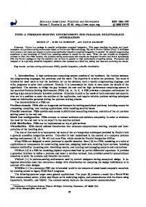
Visualization techniques have already been applied to the aircraft design problem in two ways. First, a point in multidimensional space corresponds to a rough aircraft design. It is of use to the designer to be able to see an iconic representation of the airplane shape that corresponds to a given point, such as illustrated by Figure 1. The parametric representation is transferred to physical coordinates and stored in a particular geometry format which serves as input to several of the

5


no constraint violations constraints active constraints violated range constraint landing CLmax and tip scrape tip spike constraint

Optimum 1

Figure 1. VizCraft design view window showing aircraft geometry and cross sections of the airfoil at the root, leading edge break, and tip of the wing.

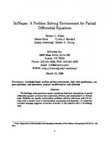
analysis methods. These physical points are then formatted as input to a plotting package. The second use of visualization illustrates the power of even simple visualizations to provide insight into a difficult problem. Figure 2 shows a section of a two-dimensional slice through the multidimensional design space using Optimum 1, Optimum 2, and a suboptimal feasible point. The remaining points are created by linearly varying the design variables between all three points. The figure is somewhat misleading in that it is normally unusual to have gathered so much information about a particular region of the design space. The relatively large number of point evaluations were performed expressly to generate the image. In Figure 2, the circles represent design points. Open circles represent feasible points while filled circles represent points that have violated some constraints. The value of the objective function is indicated by the shading. In this particular region of the design space, the objective function is relatively insensitive, resulting in a smooth “surface”, because all three points selected have similar objective function values — in the HSCT problem, numerical noise affects mostly the constraints. The curved lines on the plot represent the boundaries of four constraints. These lines are actually generated from interpolating the data achieved from the point evaluations — there do not exist simple independent equations that can be used to discriminate large sets of points as satisfying or violating an individual constraint, except as gross approximations. Designers need insight into the shape of the design space in which they work. Knowledge of the

Optimum 2

TOGW 658000 657000 656000 655000 654000 653000 652000 651000 650000 649000 648000 647000 646000 645000 644000

Figure 2. A two-dimensional slice through a multidimensional parameter space [2] using Optimum 1, Optimum 2, and another suboptimal feasible point.

constraint boundaries and variation in objective function value can allow more informed selection of optimal designs. The reason for developing this 2-D slice visualization was to gain some insight into the properties of the design space. The original motivation came from the results of an automated optimizer applied to the problem. It was known that the optimizer was sensitive to initial conditions, in that providing one starting point yielded a local optimum, while providing another starting point yielded another local optimum that was 2000 lbs lighter. Prior to creating the visualization, it was not recognized that the constraints break the design space into disjoint (at least in some hyperplanes) regions of feasible points. This insight came as a result of the visualization. Knowing whether to accept (or reject) what the optimizer tells us is important. Optimizers can have trouble with high-dimensional, highly constrained problems. Visualization in conjunction with optimization can provide understanding of the optimization process and trade-offs involved, but it also has the potential to provide guidance by an experienced engineer when the optimizer runs into trouble (such as when the gradient of the objective function is nearly perpendicular to a constraint boundary).


5

6

Design Point Visualization

In the absence of a better automated technique for solving the problem, aircraft designers would benefit from better visualization tools for helping select better designs. One approach might be a visualization system that helps better manage the information available. We have developed VizCraft, a pair of tools for visualizing HSCT designs. The first tool permits the user to quickly evaluate the quality of a given design with respect to its objective function, constraint violations, and graphical view. The second tool is an implementation of the parallel coordinates visualization [12]. Its goal is to allow the user to effectively investigate a database of designs. VizCraft provides a menu-driven graphical user interface to the HSCT design code [10], a collection of C and FORTRAN routines that calculate the aircraft geometry in 3-D, the design constraint values, and the TOGW value, among other things. Java was chosen as the programming language for development because (1) users of VizCraft needed the ability to execute it from various UNIX platforms without being concerned with user interface library installation issues, and (2) implementing it in Java would give us the ability to later cast VizCraft as an applet and leverage the Web, an important design goal of VizCraft, especially of the parallel coodinates module (described in the next section). Figure 1 shows VizCraft’s main window with a display of the HSCT planform (a top view) for a sample design. Below the planform are displayed cross sections of the airfoil at the root, leading edge break, and tip of the wing, in that order. To make observation easier, the vertical dimension of the cross sections has been magnified. Prior to developing VizCraft, designers used Tecplot to display the HSCT planform, but we decided to write a conversion routine to integrate the planform into VizCraft. This had the advantage that users would not have to run a different application along with VizCraft to view the aircraft geometry. Integration allows engineers to shift easily between a visual representation of the design and points in design space. We also added a VRML model of the HSCT planform, accessible from the menu bar. This provides the user with greater flexibility in manipulating the planform in 3-D, with ease of manipulation depending on the VRML browser used.

Figure 3. Input window for entering values of wing planform variables.

The panel to the left of the planform in Figure 1 provides access to more information about the current design point. Design variables are divided into five categories: wing planform, fuselage shape, engine nacelle location, mission variables, and tail areas. Constraints are divided into three categories: geometric, aerodynamic, and performance constraints. Clicking on the “Wing Planform” button in the main window pops up the window shown in Figure 3. This window displays the wing parameters and the values currently assigned to them. The sliders on the right can be used to modify the values of the corresponding design variables. Each time the value of a design variable is modified, the HSCT planform is immediately updated to reflect the new geometry, and so is the value of TOGW on the vertical panel. Constraints for the current design point are not automatically evaluated after each change to an input parameter, however. Since constraint evaluation is time-consuming even for the low fidelity model we are using (taking approximately 10 seconds on a dual-processor DEC Alpha 4100 5/400 under typical user loads), VizCraft evaluates constraints only when the user explicitly requests it by clicking on the “Evaluate” button shown in Figure 1. Once constraints are evaluated, the user is given feedback as follows. The colored boxes shown in Figure 1 represent information about the number of constraints violated, active, and satisfied but inactive in each category of constraints. The red


Figure 4. Geometric constraints for one design point. A red-colored box indicates a violated constraint, a yellow box indicates an active constraint, and a green box indicates a satisfied constraint.

7

Figure 5. Parallel coordinates representation of one design point using 31 vertical lines. Each vertical line represents a design parameter. The first line from the left represents the TOGW (the objective function), the second line represents the HSCT range, and the remaining 29 lines represent the design variables.

boxes indicate the number of constraints of that category that are violated, the yellow boxes indicate the number of constraints that are “active,” (i.e., close to a constraint boundary), and the green boxes indicate the number of constraints that are satisfied and inactive. Clicking on the “Geometric” Constraints button pops up the window shown in Figure 4. This window lists the geometric constraints for the current design point, and a colored box next to each one indicates if it is violated (red), active (yellow), or inactive (green).

6

Parallel Coordinates

The tool described in the previous section provides a visualization of the aircraft derived from a given design vector, and also provides a convenient view of constraint violations. However, it does not help designers with the more difficult task of understanding how a proposed design compares with other designs. This task is complicated by the high dimensionality of the problem, and the resulting difficulty in visualizing or comprehending the multidimensional design space. Few visualization techniques provide an adequate visualization of high-dimensional spaces. Since all dimensions are equally important for the HSCT design, and since we do not know where in the design space lies the region of optimal design, we cannot afford to use techniques that suffer from data hiding.

Figure 6. Parallel coordinates representation of 68 constraints for one design point. Horizontal lines split the vertical lines into three regions: satisfied (green), active (yellow), and violated (red).

One method of visualizing multiple dimensions multidimensional space is based on the concept of parallel coordinates [12]. A parallel coordinates visualization assigns one vertical axis to each visualization variable, and evenly spaces these axes horizontally, as shown in Figure 5. This is in contrast to the traditional Cartesian coordinates system where all axes are mutually perpendicular. By drawing the axes parallel to one another, one can represent points in much greater than three dimensions. In our application, potential visualization variables (equivalently, dimensions) include the design variables, the objective function value (TOGW) and other derived values such as range, and the constraint values. Each visualization variable is plotted on its own axis, and the values of the variables on adjacent axes are connected by straight lines, as shown in Figure 5. Thus, a point in an n-dimensional space becomes a polygonal line laid out across the n parallel axes with n − 1 line segments connecting the n


data values. Many such data points (in Euclidean space) will map to many of these polygonal lines in a parallel coordinate representation. Viewed as a whole, these many lines might well exhibit coherent patterns which could be associated with inherent correlation of the data points involved. In this way, the search for relations among the design variables is transformed into a 2-D pattern recognition problem, and the design points become amenable to visualization. One important aspect of this visualization scheme is that it provides opportunities for human pattern recognition: By using color to distinguish lines, and by supporting various forms of interaction with the parallel coordinates system, patterns can be picked up in the given database of design points. Given the upper and lower limits on each variable, the location of a polygonal line laid out across the n vertical axes gives some idea as to where that design point lies in the design space. The number of dimensions that can be visualized using this scheme is fairly large, limited only by the horizontal resolution of the screen. However, as the number of dimensions increases, the axes come closer to each other, making it more difficult to perceive patterns. It is also important to note the flexibility of the parallel coordinates approach in that each coordinate can be individually scaled — some may be linear with different bounds, while others may be logarithmic (although logarithmic scaling is currently not supported by VizCraft). This may aid in identifying direct, inverse, and one-to-one relationships between the parameters. Scaling an individual parameter has another advantage in that it helps us in zooming into or zooming out of a subset of the region of design space represented, effectively brushing out or eliminating undesirable portions of the design space. In Figure 5, 31 values are shown mapped onto 31 vertical axes. The first axis represents the TOGW, the second represents the HSCT range, and the remaining 29 axes represent the 29 design variables. Placing the mouse cursor on one of the circles below the vertical lines will cause the “Name of field” text field to display a description of the corresponding visualization variable. The displayed range and the absolute range for the selected variable are indicated in text fields. The absolute ranges for all the design variables are obtained automatically by locating their minimum and maximum values from the given database of

8

points. Figure 6 shows the parallel coordinates system for 68 constraints corresponding to the design point shown in Figure 5. All constraint values are normalized, with the range for violated, active, and inactive values being consistent across the constraints. All values above the yellow horizontal line indicate inactive constraints, all values between the yellow and red lines indicate active constraints, and all values below the red horizontal line indicate violated constraints. By breaking up the range of constraint values into three regions, it takes little effort on the part of the designer to assess the merit of a given design point – a quick glance at the screen conveys most of the information the designer needs in order to form a judgement of the current point(s). In Figure 6, it becomes easy to graphically identify the inactive and violated constraints, and to what degree each constraint has been violated, without having to deal directly with numbers. Representing just one design point in the parallel coordinates system may help the designer quickly view the level of constraint violations, but this is little better than the view provided by the singlepoint VizCraft tool. The real purpose of parallel coordinates in VizCraft is to allow the designer to browse a database of design points. We illustrate this process with a database of 1500 design points selected uniformly from the entire design space. When this database is rendered, it appears as shown in Figure 7. From this mass of data, one can use VizCraft’s visualization controls to extract patterns. Each polygonal line (representing one design point) is assigned a color based on the value of a particular visualization parameter. In Figure 7, the value used to determine the color is TOGW. Thus, as lines span across the vertical axes, one can identify those design points for which the TOGW is high or low. The design point with lowest value of TOGW is assigned a yellow color, the one with the highest value is assigned a black color, while the color for all the other design points is a linear interpolation between yellow and black. Since the design objective is to minimize the TOGW, the designer might initially be interested in lines rendered in yellow. However, the primary purpose of the parallel coordinates tool is to allow the user to investigate correlations between various visualization parameters, independent of the specific application context. For example, it may prove equally


useful to the designer to discover that certain design variable ranges are associated with bad designs as it is to discover that other ranges are associated with good designs. Looking at Figure 7, one can already see from the color gradation that the sixth axis from the right is directly related to the first axis. It so happens that the sixth axis from the right represents the weight of the flight fuel in lbs, which affects the TOGW directly. One can also observe that the second axis from the left is also mildly correlated to the TOGW and flight fuel. This axis represents the range of the aircraft in nautical miles, which must be directly proportional to the amount of fuel added. Even though these particular relationships are obvious (once the viewer has an understanding of the parameters involved), they give us a good start into understanding how to extract patterns from the data.

7

Visual Data Mining

A display of the full database such as shown in Figure 7 is typically too overwhelming to gain any real understanding of the data. The real strength of the parallel coordinates tool in VizCraft is the capability it provides for exploring the database. In this section we explain how the user can interact with the system “visual cues” [14] that will help in visualizing the data set in n-dimensional space. Looking at Figure 7, notice that there is a circle above each vertical axis, and that only the first one on the left is shaded. The shaded circle indicates the visualization variable that is currently “driving” the gradation of color across the parallel coordinates. For example, in Figure 7, TOGW is driving the color gradation. The user can select any visualization variable to drive the coloring by clicking inside the circle over the corresponding variable’s axis. Clicking on the fifth circle we see that that variable happens to share a direct relationship with the seventh visualization variable (Figure 8). This shows that a clever selection of color drivers can help us extract patterns from the data set — patterns which are otherwise hidden underneath the volume of data. Such patterns must exist in the data set, because 1500 points in 29 dimensions is a very sparse experimental design. A uniform sampling would contain at least 229 ≈ 109 points, as explained in Section 3.

9

The user’s ability to recognize patterns in the parallel coordinates representation can be greatly affected by the sequence in which the axes are placed. For example, it is easier to perceive relationships between two adjacent axes than if the two axes are placed far apart. VizCraft allows the user to rearrange the axes. The user simply clicks on the circle above the axis to be moved and drags it to the new position. As an example, to insert the jth axis between the ith and kth axes, the user must click on the circle located above or below the jth vertical line, drag the mouse pointer and release it somewhere between the ith and kth vertical lines, e.g., inserting the seventh axis before the sixth axis in Figure 8 results in Figure 9. It brings up clearly the one-to-one relationship shared by the fifth and seventh design variables. This rearrangement must be done with the reorder option set to “insert”. If the reorder option is set to “swap”, then one axis can be swapped with another by clicking and dragging one circle onto another. While showing a large number of design points can be helpful in generating patterns that may be of interest to the researcher at a holistic level, individual design points cannot be distinguished when too many are displayed at once. To allow clear views of individual design points, the user may wish to select from this design space a subregion of interest, or a subregion that meets certain criteria. For example, the user may wish to eliminate all design points for which TOGW is greater than 700, 000 lbs, or eliminate those points for which the range of the aircraft is less than 4,000 miles. The goal is to allow the user to gain some understanding of spatial relationships in n-space by selecting all data points that fall within a user defined set. This technique of graphically selecting or highlighting subsets of the data set is called “brushing” [15]. VizCraft makes it easy to extract regions of interest from the design space. For example, to select a region for which TOGW lies within a certain range, the user can select the circle below the TOGW axis, and then enter the range in the “zoom from” and “zoom to” textboxes. This eliminates all design points for which the value of TOGW does not lie within this range. The axis for TOGW is recalibrated to this new scale, while all other axes retain their calibration. Alternatively, the user can click on any axis, drag the mouse pointer up or down, and release it to zoom into a region of interest. Figure 10 shows


10

Figure 7. Parallel coordinates representation of 1500 design points selected uniformly from the entire design space.

Figure 9. A clever rearrangement of the design variables brings up a one-to-one relationship between two variables in the data set.

Figure 8. A clever selection of the “color driver” variable highlights a relationship between two visualization variables.

Figure 10. Result of brushing out design points lying outside a certain range of TOGW.

the result of zooming into a region of low TOGW. The text fields at the bottom indicate that there are only four design points lying in the region of interest, and that the remaining 1,496 points have been discarded. Since we are interested in designs that yield low values for TOGW, we can now observe other design variables in this design subspace. Perhaps this will allow the designer to gain insight regarding what values of these variables, or what combinations of values of these variables, produced low values of TOGW. Figure 11 shows the set of constraints corresponding to Figure 10. VizCraft provides applicationspecific visualization options related to constraint violations. The “no color” option indicates that all the polygonal lines are rendered in the default color. The “all” option indicates that the polygonal lines are colored using a rule that if any constraint is violated for a particular design point, that design point must be rendered in red. If

all constraints are satisfied for a particular design point, that design point is rendered in green. In Figure 11 there is no design point that satisfies all constraints. A third option, the “selective” coloring option, assigns a color to each polygonal line on the rule that all points for which the selected constraint is violated are colored red, those points for which that constraint is active are colored yellow, and those points for which that constraint is satisfied are colored green. As in the case of design variables, the user can select any constraint to drive the coloration by clicking on the oval on top of the vertical line corresponding to that constraint. In Figure 12, coloring is being driven by the forty-second constraint from the left (i.e., No engine scrape at landing angle-of-attack). Out of the four cases displayed, this constraint is satisfied once, is active once, and is violated twice. This coloration scheme can give an idea of the troublesome constraints, ones that are usually violated. Unlike the other visualization variables,


Figure 11. Constraints for the four design points shown in Figure 10.

Figure 12. Constraints for the four design points shown in Figure 10, with selective coloring.

the constraint values lying beyond the range of the vertical lines are truncated. This becomes necessary to maintain the positions of constraint boundary lines, i.e., the horizontal red and yellow lines. Finally, VizCraft gives the user an opportunity to click and highlight any one of the design points. To highlight a design point, the user must click at a point where a polygonal line intersects a vertical axis. Highlighting is done by assigning a bright color to the design point of interest. The highlighted point can also be viewed in its iconic representation in the main window (as in Figure 1) by clicking on the “View” button.

8

Concluding Remarks and Future Work

This paper presented VizCraft, a program for visualizing HSCT designs using a system of parallel coordinates. The implementation of parallel coordinates into VizCraft allows the user to visually manipulate the design space while searching for patterns, and to eliminate portions of the design space from consideration by carefully selecting regions of interest. However, an intuitive feel for this application of parallel coordinates can only be realized with some practice, just as an in-

11

tuitive feel for Cartesian representations is developed through usage and practice. While implementing parallel coordinates in VizCraft, special consideration was given to two aspects: user interactivity for allowing interactive data exploration, and modularity, which is necessary for adapting the system in the future to the needs of different applications, not just those specific to HSCT design. The parallel coordinates module in VizCraft has been used to display multidimensional data sets for other application areas as well, provided the data file supplied to it is in the required format. By integrating both computation and visualization facilities, and making them accessible from a high-level user interface, VizCraft has helped HSCT designers be more productive in a number of ways. The interface has streamlined the practice of exploring the effect of design variable combinations on aircraft performance for regions of the design space that have not previously been investigated. Where the designer originally had to manually change design variables in a file, run the analysis code, and then observe the results in a separate plotting package, VizCraft is able to perform these operations with a few clicks of a button. The data mining capabilities of VizCraft have proved beneficial when large databases of HSCT performance data are available. Through the use of colored driving variables and brushing techniques, designers were able to visually correlate different design variable combinations and/or patterns that resulted in either very good or very bad aircraft performance. The current implementation of VizCraft consists of two parts: a GUI for the HSCT code, and a visualization module. While this is a complete application in itself, the current implementation is missing two important features. Possibilities include (1) remote access via the WWW, and (2) integrating optimization capabilities. The World Wide Web provides opportunities for making visualization techniques available to the general public. The necessary components to access the Internet and the WWW are already available to the public and widespread. Java offers the required functionality to design the user interface and communication between a client and a server. Providing a Web-based environment to VizCraft will offer several benefits: it will enable a wider class of users to access it away from their workplaces, and from a variety of platforms. All pro-


12

cessing can be done on the server end, so users of VizCraft will not need to worry about software installation issues at the client — anybody with a Java-enabled Web browser and an Internet connection will be able to execute VizCraft.

[7] A. Messac and X. Chen. Visualizing the optimization process in real-time using physical programming. In 7th AIAA/USAF/NASA/ISSMO Symposium on Multidisciplinary Analysis and Optimization, pages 55–66, St. Louis, MO, AIAA-98-4708, September 1998.

VizCraft does not incorporate any optimization tools currently being used for the HSCT design. Integrating an optimizer like the Design Optimization Tools (DOT) [16] with VizCraft would greatly increase its power and utility. With the integration of an optimizer, users could potentially provide an acceptable range for any of the design parameters, specify which of the output values to minimize or maximize, and observe, and possibly alter, the optimization run as it is being executed.

[8] G. Kingsley, V.J. Harrand, and C. Lawrence. A visual computing environment for computational aerosciences. In Proceedings of the 1996 Computational Aerosciences Workshop, pages 331–338, NASA Ames Reseach Center, 1996.

9

Acknowledgements

This work was supported by NASA Grant NAG2-1180, NSF Grant DMS-9625968, and AFOSR Grant F496320-99-1-0128.

References [1] K. Brodlie, L. Brankin, G. Banecki, A. Gay, A. Poon, and H. Wright. GRASPARC – a problem solving environment integrating computation and visualization. In Proceedings of IEEE Visualization ’93, pages 102– 109. IEEE Computer Society Press, 1993. [2] D.L. Knill, A.A. Giunta, C.A. Baker, B. Grossman, W.H. Mason, R.T. Haftka, and L.T. Watson. Response surface models combining linear and euler aerodynamics for supersonic transport design. Journal of Aircraft, 36(1):75–86, 1999. [3] E.N. Houstis, E. Gallopoulos, R. Bramley, and J.R. Rice. Problem-solving environments for computational science. IEEE Computational Science and Engineering, 4:18–21, 1997. [4] R.P. Weston, J.C. Townsend, T.M. Edison, and R.L. Gates. A distributed computing environment for multidisciplinary design. In 5th AIAA/NASA/ISSMO Symposium on Multidisciplinary Analysis and Optimization, pages 1091–1097, Panama City Beach, FL, AIAA-94-4372, September 1994. [5] S.S. Tong, D. Powell, and S. Goel. Integration of artificial intelligence and numerical optimization techniques for the design of complex aerospace systems, AIAA-92-1189, February 1992. [6] M.S. Eldred and W.E. Hart. Design and implementation of multilevel parallel optimization on the Intel TeraFLOPS. In 7th AIAA/USAF/NASA/ISSMO Symposium on Multidisciplinary Analysis and Optimization, pages 44–54, St. Louis, MO, AIAA-984707, September 1998.

[9] G. Kingsley, J. M. Siegel Jr., V. J. Harrand, C. Lawrence, and J. J. Luker. Development of a multi-disciplinary computing environment (MDICE). In 7th AIAA/USAF/NASA/ISSMO Symposium on Multidisciplinary Analysis and Optimization, pages 251–260, St. Louis, MO, AIAA-98-4738, September 1998. [10] J. Dudley, X. Huang, P.E. MacMillin, B. Grossman, R.T. Haftka, and W.H. Mason. Multidisciplinary optimization of the high speed civil transport, AIAA95-1024, 1995. [11] E. Cluff, R.P. Burton, and W.A. Barrett. A survey and characterization of multidimensional presentation techniques. Journal of Imaging Technology, 17(4):142–153, 1991. [12] A. Inselberg and B. Dimsdale. Parallel coordinates: A tool for visualizing multi-dimensional geometry. In Proceedings of IEEE Visualization ’90, pages 360– 375, Los Alamitos, CA, October 1990. [13] J. Assa, D. Cohen-Or, and T. Milo. Displaying data in multidimensional relevance space with 2D visualization maps. In Proceedings of IEEE Visualization ’97, pages 127–134, Phoenix, AZ, October 1997. [14] A. Inselberg. Multidimensional detective. In Proceedings of IEEE Symposium on Information Visualization (InfoVis ’97), pages 100–107, Phoenix, AZ, October 1997. [15] M. O. Ward and A.R. Martin. High dimensional brushing for interactive exploration of multivariate data. In Proceedings of IEEE Visualization ’95, pages 271–278, 1997. [16] Vanderplaats Research & Development, Inc. DOT users manual, version 4.20. Colorado Springs, CO, 1995.