1
A QUANTITATIVE MODEL OF DYNAMIC VISUAL ATTENTION Neville Moray Department of Psychology, University of Surrey Guildford, Surrey United Kingdom Toshiyuki Inagaki Institute of Information Science and TARA Center, University of Tsukuba Tsukuba Japan
Abstract A mathematical model of dynamic visual attention is presented. The purpose of the model is to allow prediction of the direction of attention in dynamic real-time real-world tasks, not to explain the nature of attention. It is a predictive performance model, not a process model and is applicable to a range of tasks from eye movements scanning the environment to accessing multi-page computer displays. The variables and parameters of the model are derived from past research on sampling behaviour and include all the major factors which have been shown the affect the direction of attention. Short Title: Dynamic Visual Attention Keywords: Attention, monitoring, sampling theory, vision.
Contact: N. Moray, 17 Avenue des Genets, 06520 Magagnosc, France.
[email protected]. or Toshiyuki Inagaki, Institute of Information Science and TARA Center, University of Tsukuba, Tsukuba, Japan.
[email protected]
2
INTRODUCTION. In many tasks a human observer must dynamically allocate attention over a complex array of sources of information each of whose values vary as a function of time and which are characterised by varied dynamics and different degrees of importance. How may we model such behaviour? There is disagreement in the literature as to whether attention is fundamentally a single channel mechanism (Broadbent, 1958) or is supported by multiple resources that can be used (to some extent) in parallel (Wickens, 1992) , but there are many real-time real-world tasks where we must treat monitoring, (the distribution of attention over sources of information) as a sequential single-channel process. For example, if the human-machine interface of a complex system consists of many pages of computerised displays, only one of which can be seen at a time, attention must dynamically be redirected by calling up the appropriate pages sequentially. If conventional visual displays are used in a large control room, observers must redirect their direction of gaze so that the fixation point passes sequentially from one source of information to another. When driving a car, attention is distributed over the environment by eye and head movements. The present paper describes a model for the sequential allocation of attention in such situations. Furthermore, while multiple resource models have been able to explain experimental data after the fact, they have not been able to predict the moment to moment distribution of attention in rich dynamic environments, whereas several single channel models have been proposed, based on the dynamics of eye movements (Moray, 1986; Corker, 1998). To optimally support dynamic attention we need a model which predicts which source of information should next be fixated, and if possible at what time that fixation will occur1. The problem of dynamic attention speaks directly to the solution of practical problems. If we can predict the dynamics of attention we will be able to identify cases where the observer will be overloaded, and can then design a support system which may be should be particularly compatible, since its properties can be made to complement those of the human observer. There is also a theoretical concern: during the last 50 years several models and many papers have appeared which describe research on monitoring, visual dynamic attention, eye movements, and supervisory control (for reviews see Moray, 1986, 2005). The time seems appropriate to integrate that work into a unified model of attention.
PART 1. A REVIEW OF RESEARCH ON DYNAMIC VISUAL ATTENTION The model we propose is based on that outlined by Moray (1999a), which was in turn derived from that of Carbonell (1966). Consider a situation where the observer is monitoring a (multidimensional)
3
space in which there are many Entities (E1,E2,...,En) which must be monitored. Taken together the values in this E-vector define the state of the systm. Entities may be echoes on a radar display, video images from a remote camera, features representing the surrounding environment whether artificial (instruments, gauges) or natural (cars on a street, enemy aircraft), printed messages on a screen, alarms, etc.. The Es have properties that change over time, variables such as position, velocity, intent (attacking, overtaking, etc.), brightness, or verbal content. A general statement of the observer's task is that the latter must monitor these properties to keep track of the state of each entity so as to identify the moment to moment state of the system and to notice any significant or unexpected change in each E, and the appearance of new Es and the disappearance of existing ones. We adopt as a basic framework the notion of constraint boundaries and uncertainty. We assume that for every variable there are certain values that must not be exceeded. For example, a car should not cross the lane boundary if there are double lines; pressures should not exceed safe limits in industrial processes; temperatures should be neither too high nor too low in the steam generator of a power plant; hostile aircraft should not come within a range where their missiles can threaten the observer, etc.. We assert that the fundamental task of dynamic visual attention is to notice the approach to, or the crossing of, such constraint boundaries. We call the situation where a variable crosses a constraint boundary an accident. Some intuitive qualitative remarks are relevant. Es with slow dynamics need be observed only rarely, those with fast dynamics frequently, while unexpected events should attract attention and cause an “interrupt driven” redirection (capture) of attention. Es with dangerous or valuable consequences should be monitored more frequently, and those represented by unreliable data should be monitored more frequently. In the following development we make use of well-founded empirical generalisations from laboratory or industrial research. Individual findings are combined to form an integrated model of the dynamics of attention, although to date no single experiment has combined all the findings. We believe the components of the proposed model have already been validated since they represent published empirical findings. We summarise the research that define the requirements of a model, and then present a quantitative model of expert, highly practised, observers, that assumes that observers have a good knowledge of the statistical dynamics of the processes being observed. The monitoring problem is defined as the following: Determine when the next observation of each entity should be made (determine the sampling interval, instant, and object). For each entity determine whether the entity state vector value is satisfactory on the basis of the sample. If the entity state vector is unsatisfactory, determine what action to take, including changing control
4
from manual to automatic or automatic to manual either for the total control or for a subset of variables, initiating action or further monitoring, etc.. Respond to the sudden appearance (and perhaps disappearance) of entities from the set under observation by at least one observation. We refer to the act of directing attention to a source or entity as sampling or monitoring. We do not explicitly treat the problem of sustained watch-keeping or vigilance. Properties of the observer We model the observer as a single channel discrete sampling observer with memory. To so characterise the observer is from a design perspective conservative, which is desirable. If the assumption is incorrect, and some more parallel model of attention is correct, then performance will be better than that of the proposed model. The observer's long-term memory contains representations of the properties of entities based on past experience which can be thought of as a series of dynamic mental models. Such information can be called into working memory as required. The mental models also serve to set parameters at the beginning of a watch-keeping period. Each time an entity is observed the observer’s mental models of the state of the entity and its properties (state vector) are updated. Origins of uncertainty We agree with Senders (1964, 1983) that the basic use of attention in dynamic environments is to reduce observers’ uncertainty, and we define uncertainty as the position of variables with respect to their constraint boundaries. If it is known that no variable will cross its constraint boundary, (even those that characterize entities which are currently absent but which may from time to time appear,) then there is no reason to pay attention to the system. Uncertainty arises from three sources, two exogenous and one endogenous. The first exogenous source of uncertainty is the possibility that new entities will enter the system or old ones disappear. The description of the state space is non-stationary. Such changes often cannot be predicted, and hence the observer must be sensitive to their occurrence, and gross changes in the properties of the state space must cause an interrupt which directs attention to the new entity. Everyday experience and research on the orientating reflex suggests that sensitivity to change is a property of the brain which is in-built as a result of evolution. Many texts note that sudden changes, or the appearance of “salient” stimuli tend to capture attention, but we know of no quantitative model of salience, and no general quantitative model of “sudden change”. We will suggest one below. Of all the properties of the model this is the one which is least supported by prior research.
5
The second exogenous source of uncertainty is the dynamics of entities. For example an entity such as a vehicle that is attempting to follow a prescribed course is subject to perturbations caused by the environment, and to variation caused by inadvertent inaccuracies in the behaviour of the (human or automatic) controller, and these perturbations must be offset by the controller of the vehicle. Often the time history of a variable can be approximated, at least over a useful length of time, as a continuous zero-mean Gaussian distribution of the amplitude of a function with a bandwidth determined by the rate of change of the variable and the power spectrum of the perturbations. The uncertainty associated with the variable dynamics can then be precisely defined using Information Theory (Shannon and Weaver, 1948; Sheridan and Ferrell, 1974). Such an approximation can often be used for the time history of temperatures, pressures, and a variety of other variables. The approach can be generalised by using other functions than the Gaussian. The set of variables which together describe the time history of a multi-variate entity comprise the entity’s state vector. Further characteristics of the entity state vector give rise to other aspects of uncertainty which will be discussed below. Throughout, the word velocity and the phrase rate of change should be regarded as equivalent. In many tasks the main endogenous source of uncertainty is forgetting. In general this is true of all systems with very slow dynamics. Suppose that at time t, the observer observes entity E and establishes its state vector (identity, position, velocity, etc.). Because of the need to monitor other entities, the observer then ceases to observe E. As time passes the memory of the observation on E fades or becomes corrupted, and hence the uncertainty of the observer about the value of E increases, until at some time t + τ the endogenous uncertainty passes a threshold and the observer takes a new observation of E (Moray, Richards and Low, 1980; Moray, Neil and Brophy, 1983). There are other endogenous sources of uncertainty associated with imperfect knowledge or imperfect mental models, but these will be discussed later. Empirically known properties of attention control The properties of entities and observers known from the literature to be important in determining dynamic attention are shown in Table 1. A review of many of the early results can be found in Moray (1986). We consider briefly each item in Table 1. We assume that the observer is highly experienced and has a perfect knowledge (not necessarily accessible to consciousness) of the relevant statistical and mathematical properties of variables, acquired as a mental model in long term memory as a result of extended practice at the tasks.
6 INSERT TABLE 1 ABOUT HERE 1. Interrupts
Although there is an extensive literature on warnings and alarms (see, e.g. Laughery, Wogalter, & Young, 1995), there is remarkably little quantitative modelling of their effects. It is commonly stated that a sudden change in a portion of a display will attract attention provided that it is large. This property is often referred to as “salience”, but there seems to be no general quantitative model of salience. To model dynamic attention it is important to include the capturing of attention by interrupts, and we therefore propose in the model that the rate of change weighted by the magnitude of the change is the property which attracts attention. 2. Bandwidth and Temporal Uncertainty The importance of bandwidth and temporal uncertainty was modelled by Senders and his associates in the early 1960s, and the validity of this approach has been confirmed subsequently on numerous occasions (Senders, Elkind, Grignetti and Smallwood, 1965; Senders, 1964, 1983; Sheridan and Ferrell, 1974; Parasuraman, Molloy and Mouloua, 1993; Leermakers, 1995). Related field studies were reported by Iosif (1968, 1969a, 1969b, Moray, 2005). Our proposed model will not use these factors in exactly the way they were used by Senders (1964) in his classic study, but are implicit in the mathematics of our model of uncertainty. The work of Senders will be discussed here to provide a context free background, because his work provides a clear presentation of general mathematical properties of abstract sampling theory in relation to dynamic uncertainty. In general, if a variable has high frequency dynamics, the temporal uncertainty of its value requires that it be monitored frequently. If the variable can be characterised as a limited bandwidth zero mean Gaussian function of time, then the Nyquist Sampling Theorem and Shannon’s Information Theory for continuous variables define the optimal sampling frequency and the duration of a sample (Shannon and Weaver, 1948; Sheridan and Ferrell, 1974). The Nyquist Theorem states that if a process is bandwidth limited to W Hz, then if at each sample the instantaneous value of the amplitude of the variable is observed, it is necessary and sufficient to sample it at 2W times per second to be able to reconstruct the function. If the observer can estimate the rate of change as well as the position of the observed variable, then the frequency of sampling can be reduced to W samples per second (Senders, 1983). If the root mean square (rms) amplitude of the signal (or the required precision of the observation) is S, and the rms of the noise is N, then the information per observation is log2
!!! !
bits and the duration of the observation will be proportional to this value (Sheridan
7
and Ferrell, 1974). Note that the duration of observation is important: in principle a lengthy observation of one variable will delay an observation of another variable. It then limits the rate at which attention can be switched. In some (but not all) cases the duration of an observation can be identified with the duration of a fixation. Empirical evidence suggests that attention switches in the sense of redirection of fixations are seldom made at a rate of more than 2 – 3 times a second and usually at a much slower rate (Boff and Lincoln, 1988; Moray, 1986). Changing the direction of attention by changing fixation using eye movements is probably the most rapid way to switch attention. Other limits on the switching rate may be technical, for example the time it takes to call up a new page on a computer display. We shall not discuss the problem of modelling fixation duration in detail. For some classes of signals Information Theory metrics can be used (Senders, 1964; Sheridan and Ferrell, 1974), and for others GOMS estimates (Card, Moran and Newell, 1983). Information Theory predicts that if the quality of the information derived from sensors is poor, that is, the signal-to-noise ratio is low, then the duration of an observation will increase, thereby delaying the opportunity to sample another source. An alternative formulation of this point is that the duration of an observation will increase if the required accuracy with which the value of the variable is measured is increased (the tolerable error of estimation is decreased). There appears to be no direct study of this problem, since in Senders’ original work on instrument monitoring (see Senders, 1964) he took care that the bandwidths were so low that there would not be any significant probability of simultaneous demand from more than one source. Furthermore, since the S/N ratios were identical for all the instruments, it was expected that the fixation duration would not differ among them, which Senders found to be the case. In many displays Es cannot be described as zero mean Gaussian functions. For example, a variable may be discrete, taking values (0,1), such as a light being on or off, red or green. In such cases there is still a relation between the frequency of the occurrence of discrete changes of state and the sampling interval. In general, the higher the frequency of changes in E, the more frequently the observer should sample it. There may be other constraints, such as the scan rate of a radar, which determines a periodic minimum interval at which new information can arrive. In the case of a series of discrete events, (such as the arrivals of cars at an intersection, or the transmission of radio IFF messages,) it may be possible to characterise the times of arrival of changes in E by some statistical distribution such as a Poisson distribution or a Markov process. Carbonell’s model (Carbonell, 1966) assumes a particular function to describe the temporal dynamics, but there is no inherent limit on the choice of function, and different functions should be used as appropriate to different variables. 3. Proximity to constraint boundaries
8
Senders et al. (1965) suggested that the attention sampling interval when monitoring a bandwidth limited Gaussian source could be related to the proximity of the variable to its constraint boundaries. Carbonell (1966; Carbonell, Ward and Senders 1968) extended their ideas, suggesting that most entities cannot be characterised by Gaussian signals with a fixed mean and standard deviation. He suggested that a more general model should include variables whose mean and standard deviation vary with time, and also that provision should be made for the fact that in many tasks the observer must restore the variable to its set point (original mean) when it is found to be diverging. In his model costs are associated with the violation of constraint boundaries: the purpose of monitoring is to avoid the costs incurred by variables crossing their constraint boundaries, or equivalently in some circumstances by a variable departing from a set point. Leermakers has empirically verified Carbonell's predictions about sampling intervals in a laboratory setting (Leermakers, 1995), and van Westeren (1999) has applied the model in a field setting of ship pilotage. Moray, Richards, and Low (1980) and Moray, Neil, and Brophy, (1983) were able to predict fighter controller mental workload and scan patterns using a closely related model. 4. Trust, Reliability and quality of sensor information There are several empirical studies of the effect of reliability on attention. For example Muir (1994) ,Muir and Moray (1996) and Leermakers (1995) investigated the effect on sampling behaviour of unreliability in displays and controls. Several studies report that the less reliable the displays, the more frequently they are sampled. Parasuraman, Molloy and Singh (1993) found that a process is monitored more frequently as the probability of faults increases in a task involving a mixture of tracking, and monitoring. Muir examined the relation between the reliability of displays, the reliability of controls, subjective trust in the quality of automation, and the frequency of monitoring. In a simulated continuous process control task she found that the larger the magnitude of faults, the more frequently was the faulty component monitored. From her work it appears that the probability of monitoring entity Ei is given by 𝑝 𝐸! = 𝑎 + 𝑏𝑒 !!! where ri is the subjectively perceived reliability of the display showing the value of xi, the variable of Ei which is monitored. We assume that reliability is experienced as the proportion of occasions on which the observer measures a variable and subsequently confirms that the measured value was correct.
𝑟 𝑥! =
𝑛𝑢𝑚𝑏𝑒𝑟 𝑜𝑓 𝑐𝑜𝑟𝑟𝑒𝑐𝑡 𝑜𝑏𝑠𝑒𝑟𝑣𝑎𝑡𝑖𝑜𝑛𝑠 𝑡𝑜𝑡𝑎𝑙 𝑛𝑢𝑚𝑏𝑒𝑟 𝑜𝑓 𝑜𝑏𝑠𝑒𝑟𝑣𝑎𝑡𝑖𝑜𝑛𝑠
9
5. Forgetting Several experiments suggest that observers sample too frequently when monitoring very low frequency processes. This apparent “scepticism” appears to be due to forgetting. Suppose an observation has been made on some entity Ei. Then as time passes the observer will become increasingly uncertain about the value of Ei. Empirical research (Moray, Synnock and Sims, 1973; Moray et al. 1980, 1983) suggests that a variable will be sampled about once every 7 -10 seconds even if its value does not much change. This can also account for the over-sampling of very low bandwidth variables discovered by Senders (1964, 1983). In general, when an observation is made, there will always be some minimal "observational error" which limits the accuracy of the estimate of the value of the observed variable. A general way to represent the impact of forgetting on attention dynamics is to assume that at each observation the observer reduces uncertainty to the value of observation error, and then to assume that all estimates of error become noisy with the passage of time using a function similar to that found by Moray et al. (1980, 1983). They modelled forgetting as a random walk that caused the uncertainty about value of a variable to increase with time. The probability of forgetting is also a source of cost, since as the observer forgets (becomes more uncertain of) the location of the state variables of E in state space, it becomes increasingly likely that a constraint boundary will be violated by that variable before the next observation. 6. Payoffs: Costs and Rewards. The experiments of Kvalseth (1977) show that if the act of making an observation is costly, then observations are made less frequently, while if the reward of making an observation is high observations are made more frequently. His experiments used cash costs and rewards. 7. Effects of control actions. We now consider the sampling model in the context of controlling a variable that is observed to be close to or beyond a constraint boundary, as described by Carbonell (1966), who suggested that on finding that a variable has diverged from the set point to an unacceptable extent a control action is initiated, and the latter drives the variable back asymptotically towards the set-point. Since this resetting is deterministic, we assume that there is no need to again observe the variable until such time as it is expected to be close to its set-point, when its value may begin to diverge
10
again. Crossman and Cooke (1974) however reported that following a control action experienced operators take a check sample when a variable has reached about 80% of its final (set point) value. This can be incorporated into the model of dynamic visual attention by assuming that operators have in their mental model a representation of the time constants of the asymptotic return to the set point. When control is exercised on a continuous variable, it is deleted from the list of variables to be sampled until it has returned 80% of the way to the set point, that is, for a period equal to about 1.6 times the time constant of the exponential return. Similarly, a discrete variable that is reset in a single step is deleted from the list for the expected value of its discrete (Poisson, Markov, etc.) time function.
8. Mental models and the initialisation of parameters. We assume that observers have long term mental models which enable them to set the parameters of the scheduling model when starting a monitoring task. During the long practice which makes the observers into experts at attending to the processes being monitored, operators build up, for the most part unconsciously, mental models of the dynamics and statistics which characterise the processes, entities and variables being observed. By “mental models” we mean mappings of the dynamics, statistical parameters, and costs and rewards which characterise the environment being monitored (Moray, 1997, 1999b). These include the time constants of the effects of control actions. These models reside in long term memory, and can be thought of as related to “scripts” and “frames” (Minsky, 1975; Schank and Abelson, 1977), although they may be analogue representations rather than discrete digital models. When operators begin a monitoring task, they access mental models of past experience of scenarios containing similar entities and initialise the attention scheduling. Using frames and scripts from mental models of the scenario for default values for probabilities, costs, etc., operators set all parameters which are required to schedule observations for all entities.
INSERT FIGURE 1 ABOUT HERE
11
PART 2. MODEL DESCRIPTION Figure 1 summarises the information and control flow in the proposed model. We now describe a mathematical model for the dynamic allocation of attention incorporating the empirically validated research described in the first part of this paper.
Glossary
αj
monetary cost associated with an accident of an entity that occurs when its state variable j passes the constraint boundary Lj
ρj
monetary cost to perform a reset action for an entity responsible for state variable j
µj
monetary cost to monitor state variable j
Θ
cost indifference threshold that defines a “negligible” amount of cost
Lj
limit which must not be passed, a constraint boundary
Mj
threshold for a reset action for entity responsible for state variable j
t
time
vj (t) = 𝑃 𝑥! 𝑡 > 𝑀! 𝑥! 𝑡!! = 𝑥!!
conditional probability that state variable j is above its
action threshold at time t, given it was last observed at time tj0 when it was observed that xj(tj0 ) = xj0 wj(t) = 𝑃 𝑥! 𝑡 > 𝐿! 𝑥! 𝑡!! = 𝑥!!
conditional probability that state variable j is above its
constraint limit at time t, given it was last observed at time tj0 when it was observed that xj(tj0 ) = xj0 xj(t)
value of state variable j at time t
zj(t)
zero-one variable, zj(t) = 1 if state variable j is monitored at time t, zj(t) = 0 otherwise
𝜉!!
variance of observation noise on state variable
Let there be m entities to be monitored. An entity is composed of one or more state variables, such as position, velocity, direction, colour, brightness, etc.. Let n be the total number of state variables required to describe m entities.
12
Let xj(t) be the value of state variable j at time t. Among variables 1 through n, we assume that at most one variable can be monitored at time t. Monetary cost to monitor state variable j is µj. Note that it may be that no state variable is monitored at time t, if monitoring at that moment is judged to be cost-ineffective. (See below.) State variable j may change its value dynamically as time goes by, and may deviate from values expected under normal operating conditions. We say an accident is said to occur when the state variable passes its constraint boundary Lj. The monetary cost associated with the accident is αj. Associated with each variable is an action threshold. When state variable j passes the action threshold Mj which is set lower than Lj and this occurrence is observed by the monitor, the monitor will act on the entity that is responsible for state variable j. The reset action will bring the state variable back to its completely normal value (set-point, mean). The monetary cost for the reset action is ρj. Let tj0 be the time point when state variable j was monitored last when it was found that xj(tj0 ) = xj0 . Since then state variable j has not been monitored, and thus its current value can merely be guessed with some uncertainty. Suppose state variable j is monitored at time t. Note here that we say “time t” to represent a short time interval [t’, t”] where t belongs to the interval. We can distinguish the following two possible outcomes of the monitoring. 1. A reset action is taken, where the possibility of this happening is given by the conditional probability vj (t) = 𝑃 𝑥! 𝑡 > 𝑀! 𝑥! 𝑡!! = 𝑥!!
(1)
2. No reset action is required with probability 1- vj(t) .
(2)
Suppose state variable j is not monitored at time t. We can distinguish the following two possible cases. 1. If the state variable was not monitored in the previous time interval, its value may be already above Mj and it may pass the constraint boundary Lj. No reset action will be taken to prevent the state from passing Lj, because the state variable is not monitored at all. An accident can happen with probability
13 wj(t) = 𝑃 𝑥! 𝑡 > 𝐿! 𝑥! 𝑡!! = 𝑥!!
(3)
2. No accident occurs with probability 1- wj(t).
(4)
If state variable j were to be monitored at time t, the expected cost would be given by vj(t)ρj + µj .
(5)
On the other hand, if state variable j were not to be monitored at time t, the expected cost would be given by wj(t)αj .
(6)
Let us introduce a zero-one variable zj(t) defined by zj(t) = 1, if state variable j is monitored at time t, zj(t) = 0, otherwise. Then, the expected cost to pay with respect to state variable j at time t is represented as follows: zj(t)[vj(t)ρj + µj ] +[1 - zj(t)]wj(t)αj = zj(t)[vj(t)ρj + µj - wj(t)αj] + wj(t)αj
(7)
Which state variable is to be monitored at time t is described by the collection of zero-one variables, {z1(t), …, zn(t)}, which we call the monitoring policy at time t. The expected cost of the monitoring policy is given by ! !!!
𝑧! 𝑡 𝑣! 𝑡 𝜌! + 𝜇! − 𝑤! 𝑡 𝛼! + 𝑤! 𝑡 𝛼!
(8)
For instance, when the observer decides to monitor state variable j, the above cost expression yields the following 𝑣! 𝑡 𝜌! + 𝜇! +
!!! 𝑤!
𝑡 𝛼!
(9)
The terms in the parenthesis gives the expected cost to be paid when state variable j is monitored, and
!!! 𝑤!
𝑡 𝛼! expresses the expected cost due to accidents in state variables that are
not monitored at time t. An optimal monitoring policy at time t is determined by solving the following zero-one integer programming problem:
14
Minimize ! !!!
𝑧! 𝑡 𝑣! 𝑡 𝜌! + 𝜇! − 𝑤! 𝑡 𝛼! + 𝑤! 𝑡 𝛼!
(10)
subject to the constraints ! !!! 𝑧!
𝑡 =1
(11)
zj(t) = 0 or 1 (j = 1,….,n) The constraint
! !!! 𝑧!
(12)
𝑡 = 1 states that exactly one state variable must be monitored. The above
problem is easy to solve. All we have to do is find zk(t) with the smallest coefficient, viz., 𝑣! 𝑡 𝜌! + 𝜇! − 𝑤! 𝑡 𝛼! < 𝑣! 𝑡 𝜌! + 𝜇! − 𝑤! 𝑡 𝛼!
(13)
for all 𝑗 ≠ 𝑘. Then the optimal policy is to monitor state variable k at time t. When 𝑣! 𝑡 𝜌! + 𝜇! − 𝑤! 𝑡 𝛼! has a negative sign, which is usually the case, its absolute value 𝑣! 𝑡 𝜌! + 𝜇! − 𝑤! 𝑡 𝛼!
(14)
measures the cost-effectiveness of monitoring. The bigger the value of 𝑣! 𝑡 𝜌! + 𝜇! − 𝑤! 𝑡 𝛼! , the more cost-effective the monitoring of state variable k, because the cost of accident (k) relative to the cost of monitoring k increases with the value of 𝑣! 𝑡 𝜌! + 𝜇! − 𝑤! 𝑡 𝛼! . What happens if 𝑣! 𝑡 𝜌! + 𝜇! − 𝑤! 𝑡 𝛼! is positive? If that is the case, k should not be monitored, because the expected cost to monitor the state variable and to reset a corresponding entity when necessary, 𝑣! 𝑡 𝜌! + 𝜇! , is greater than the expected cost of an accident that may occur while not monitoring the state variable k, namely 𝑤! 𝑡 𝛼! . No other state variables need be monitored, because we already have determined that to monitor those variables is not optimal and is less costeffective than monitoring state variable k. An extreme and probably rare case in which we do not have to monitor any state variable at all is where we know definitely that, even if a state variable may pass its action threshold M, it never crosses its constraint boundary L. In this case 𝜇! which is always positive.
𝑣! 𝑡 𝜌! + 𝜇! − 𝑤! 𝑡 𝛼! is reduced to 𝑣! 𝑡 𝜌! +
15
There is another and more realistic condition when there may be no need to monitor any state variable at time t. If 𝑣! 𝑡 𝜌! + 𝜇! − 𝑤! 𝑡 𝛼! is negative but its absolute value is very small, there may be no big difference between monitoring state variable k and disregarding it. More formally, let Θ denote the cost indifference threshold that defines a “negligible cost.” Then if 𝑣! 𝑡 𝜌! + 𝜇! − 𝑤! 𝑡 𝛼! < Θ
(15)
it is not worth monitoring state variable k. No other entity needs be monitored, because the above inequality implies 𝑣! 𝑡 𝜌! + 𝜇! − 𝑤! 𝑡 𝛼! < Θ for all j such that 𝑣! 𝑡 𝜌! + 𝜇! − 𝑤! 𝑡 𝛼! < 0 . Any state variable j for which 𝑣! 𝑡 𝜌! + 𝜇! − 𝑤! 𝑡 𝛼! > 0 need not be monitored, as we have already seen in the previous discussion. Note that the probability of such occasions, where no monitoring is required, provides a measure of operator workload: the greater the probability that no monitoring is required at any time t, the lower the workload due to monitoring at that moment.
3. EXAMPLES OF APPLICATION To derive an optimal monitoring strategy we need to calculate conditional probabilities 𝑣! 𝑡 = 𝑃 𝑥! 𝑡 > 𝑀! 𝑥! 𝑡!! = 𝑥!!
(16)
and 𝑤! 𝑡 = 𝑃 𝑥! 𝑡 > 𝐿! 𝑥! 𝑡!! = 𝑥!!
(17)
for each state variable xj(t) . The uncertainty represented by these equations can arise from various sources, and such sources must be explicitly represented in the model when it is applied to real situations. We will now give examples of how this can be done. Consider first the classical Carbonell (1966) model of a zero mean Gaussian continuous function of time, such as the (somewhat unstable) flight path of a plane (Carbonell, 1966). Suppose that state variable j was monitored last at time tj0 to find that 𝑥! 𝑡!! = 𝑥!! . Then on the one hand the real behavior of j will be such that at time t its value will be 𝑥! 𝑡; 𝑡!! .
16
On the other hand we can predict the dynamic behavior of j after tj0 as 𝑥!! 𝑡; 𝑡!! , where 𝑥!! 𝑡; 𝑡!! satisfies the following initial condition claiming that the predicted behavior 𝑥!! 𝑡; 𝑡!! must coincide with the actually observed value at time tj0 : viz., 𝑥!! 𝑡; 𝑡!!
= xj0
(18)
The observer is assumed to know that xj is normally distributed with mean 𝑥! 𝑡; 𝑡!! and variance 𝜎 ! 𝑡 = 𝜎! ! 1 − 𝑢 ! 𝑡 + 𝑠 𝑡
+ 𝜉 !
(19)
where u2(t) denotes the autocorrelation function which is unity when 𝑡 = 𝑡!!" 𝑠 𝑡 a divergence function (Sheridan & Ferrell, 1974) that describes the operator’s forgetting, and ξ2 is the variance of the observation noise (that is, a measure of how difficult it is to measure the value of the observed variable). Then we have
𝑣! 𝑡 = 𝑃 𝑥! 𝑡 > 𝑀! 𝑥! 𝑡!! = 𝑥!! =
𝑤! 𝑡 = 𝑃 𝑥! 𝑡 > 𝐿! 𝑥! 𝑡!! = 𝑥!! =
! !!! ! !
! !!! ! !
! 𝑒𝑥𝑝 !!
! 𝑒𝑥𝑝 !!
−
−
! ! !! !;!!!
!
!! ! !
! ! !! !;!!! !! ! !
dy
(20)
dy
(21)
!
Reliability and Quality of Sensor Information In the above model, we have made an implicit assumption that the state variable information derived from sensors is precise and correct apart from a (generally small and random) observation noise. In some practical cases, however, reliability or quality of sensor information may not be perfect. In this section, it is shown how the model in the previous section can be generalised to cases in which sensors give imprecise information. Consider the following cases: Case 1. Sensor for a state variable fails to give any data. Case 2. Sensor gives a wrong value that is higher than the real value of the state variable. Case 3. Sensor gives a wrong value that is lower than the true value of the state variable. Case 4. Sensor is corrupted by random noise. Suppose we have found, when monitoring state variable j, that Case 1 is true. Since the sensor does
17
not transmit any data, all we can do is estimate the present state as 𝑥! 𝑡; 𝑡!! based on our best knowledge of the dynamics of the state variable and its value at the last observation. Case 2 usually yields a fail-safe result. For instance, the operator may take an incorrect reset action based on spurious information indicating that an action threshold has already been passed, or the plant may be shut down unnecessarily by wrongly believing that the state variable is about to pass its constraint boundary. Suppose some of n state variables are measured with sensors that tend to give incorrectly higher values. Then an “optimal” monitoring policy as derived by the model tends to be biased such that those state variables are monitored more frequently. Case 3 is the most dangerous. Suppose the sensor gives a reading that is lower than an action threshold, but that the state variable is actually above the threshold. If the operator did not know that, no action would be taken even when an immediate response is required. This type of delay may eventually cause an accident since not only the action threshold but also the constraint boundary may be passed unwittingly. Case 4 is the most uncertain. Sometimes the sensor gives the correct value, sometimes a value too high, sometimes a value too low, and these variations may be much larger than the usual variance of the observation noise, ξ2. How can we modify the model to cope with cases in which sensor information is not perfectly reliable? Suppose the sensor for state variable j gives an imprecise reading xj(t) that is lower than the real value. Let Rj be an adjusting constant so that Rjxj(t) will give the true value. In Case 3, it is assumed that 1 < Rj .
(22)
An optimal monitoring policy can be derived by solving the zero-one integer programming problem in the previous section, where vj(t) and wj(t) must be re-defined as follows:
𝑣! 𝑡 = 𝑃 𝑅! 𝑥! 𝑡 > 𝑀! 𝑥! 𝑡!! = 𝑥!! = 𝑃 𝑥! 𝑡 >
𝑤! 𝑡 = P 𝑅! 𝑥! 𝑡 > 𝐿! 𝑥! 𝑡!! = 𝑥!! = P 𝑥! 𝑡 >
!! !!
!! !!
𝑥! 𝑡!! = 𝑥!!
𝑥! 𝑡!! = 𝑥!!
(23)
(24)
Note in the above expressions that the action threshold and the boundary limit are re-set at lower values using the adjusting constant Rj.
18
In Case 4, Rj is not a constant but a random variable. Several monitoring policies may be considered for this case. The first is the most “pessimistic” and the largest possible value for Rj is applied in Equations (23) and (24). The second is the most “optimistic” and the smallest possible value for Rj is applied in Equations (23) and (24). The third is to disregard the sensor reading and to guess the present state based on our best knowledge of the dynamics of the state variable. The fourth policy is a more sophisticated “randomised policy” for Case 4. Suppose Rj is modelled as a discrete random variable with a discrete probability distribution 𝑝!! , . . . . . , 𝑝!! , where 𝑝!! denotes (23), we can derive an optimal monitoring policy for a case of 𝑅! = 𝑅!! . Let jk denote the state variable that must be monitored when 𝑅! = 𝑅!! . Then the randomised policy is to monitor state variable jk with probability 𝑝!! . It is straightforward to extend the above randomised policy to a case in which Rj is modelled as a continuous random variable.
The capture of attention by interrupts Assume that a displayed variable will change somewhere in the observer's visual field2. Let the monitored visual field be subjectively divided into a number of locations, S1, . . .,Sn. Let each Si potentially contain an entity Ej (j = 1,…,Ni) characterised by a set of variables (a state vector) 𝑣!! (k = 1, . . . ,Mj) such as colour, brightness, pattern, shape, etc., and let these be called v1, . . . .,vm. Let the variables associated with EI be represented as 𝑣!! etc. Then, if the observer is currently observing some part of the display other than S, the probability that the observer’s attention will be captured by a change in S where EI is located will be determined by the magnitudes and rates of change of the variables in S. If 𝑃 𝐼𝐷!!
is the probability of an interrupt-driven observation of EI, then
P 𝐼𝐷!! = c!
!! !"!" !!! !"
(25)
That is, the probability of attention being caught by sudden changes in an entity, including its sudden appearance or disappearance, is related to the sum of the rates of change of the values of its variables summed over all variables of its state vector. The constant cI can be a function of the importance of the entity EI, and can in principle scale the sum of the rates of change so as to form a mean value,
19
etc.. It is currently not known whether the way to combine rates of change is by summation, product, etc.. Empirical research is needed to make this equation more precise. In principle it should be possible to include what is known of the different sensitivities of different parts of the retina in calculating salience. Interrupt driven calls for attention are bottom-up sensory driven determinants of attention. An observation made in response to an interrupt driven call of attention will result in the observer identifying the entity if it is one that has been previously encountered, or creating a new entry in the mental model memory containing the characteristics of the observed entity if it is new. Henceforth the entity and its list of state variables will be included in the calculations of optimal sampling strategies, and hence will be included in the top-down, mental-model-driven sampling strategies.
Conclusion The model can be used for a variety of practical system design purposes - to estimate work load, to predict the probability that a particular entity will be attended at a particular time, quantitatively to estimate the probability of so-called "complacency" (Moray and Inagaki, 2001), and to evaluate the usability of control room designs and multi-page computer displays, etc.. The model is a pragmatic competence model, not a model of underlying mechanism, - what is sometimes called an "engineering" rather than a "psychological" model. In the introduction we noted that whether or not a deep theory of attention implies that attention can process information in parallel, there are many situations in "real world" tasks in which attention is constrained by the nature of the task to be sequential3. The model we present is intended to apply to such situations.
20
References Boff, K. & Lincoln, J. (1988). Engineering Data Compendium. Ohio:WPAFB. Broadbent, D.E. (1958). Perception and Communication. Oxford: Pergamon Press. Carbonell J. R. (1966). A queuing model for many-instrument visual sampling. IEEE Transactions on Human Factors in Electronics, HFE-7, 157-164. Carbonell, J. R., Ward, J. L., & Senders, J. W. (1968) A queuing model of visual sampling: Experimental validation. IEEE Transactions on Human Factors in Electronics, HFE-9, 82- 87. Card, S. K., Moran, T. P., and Newell, A. (1983). The psychology of human-computer interaction. Hillsdale, NJ: Lawrence Erlbaum Associates. Corker, K. (1998). Man-machine integrated design and analysis system (MIDAS) functional overview. In A Designer’s Guide to Human Performance Modelling. AGARD, North Atlantic Treaty Organisation, Brussells. A9-1 – A9-15. Crossman, E.R. and Cooke, F.W. (1974). Manual control of slow response systems. In E. Edwards and F. Lees, Eds., The human operator in process control. London: Taylor & Francis. 51-66 Iosif, G. (1968). La stratégie dans la surveillance des tableaux de commande. I. Quelques facteurs déterminants de caractère objectif. Revue Roumanien de Science Social-Psychologique, 12, 147-161. Iosif, G. (1969a). La stratégie dans la surveillance des tableaux de commande. 2. Quelques facteurs déterminants de caractère subjectif. Revue Roumanien de Science Social-Psychologique, 13, 29-41. Iosif, G. (1969b). Influence de la correlation fonctionelle sur parametres technologiques. Revue Roumanien de Science Social-Psychologique, 13, 105-110. Kvalseth, T. (1977). The effect of cost on the sampling behavior of human instrument monitors. In T. B. Sheridan,. and G. Johannsen, (Eds.), Monitoring Behavior and Supervisory Control, New York: Plenum. Laughery, K. R., Wogalter, M. S., & Young, S. L. (1995). Human factors perspectives on warnings. Santa Monica, CA: Human Factors and Ergonomics Society. Leermakers, T. (1995). Monitoring behaviour. Eindhoven: Eindhoven University of Technology. Minsky, M. (1975). A framework for representing knowledge. In P. Winston (Ed.) The Psychology of Computer Vision. New York: McGraw-Hill. Moray, N. (1986). Monitoring behavior and supervisory control. In K. R. Boff, L. Kaufman, and J.P. Thomas, (eds.). (1986) Handbook of Perception and Human Performance. Chapter 45. New York: Wiley. Moray, N. (1997). Models of Models of . . . . Mental Models. In T. B. Sheridan and T. Van Lunteren (eds). Perspectives on the Human Controller. Mahwah, N.J.: Lawrence Erlbaum. 271-285. Moray N. (1999a) A model of the dynamics of monitoring and function allocation in supervisory control. Technical report CBR TR 99-2. Nissan Cambridge Basic Research, Cambridge, MA. Moray, N. (1999b). Mental models in theory and practice. Attention and Performance XVII.
21
Cambridge, MA: MIT Press. Moray, N. (Ed.) 2005. Ergonomics: Major Writings. Vols. 1 – 4. London: Taylor and Francis. Moray, N. and Inagaki, T., (2000) Attention and complacency. Theoretical Issues in Ergonomic Science. 1(4), 354 – 365. Moray, N., Richards, M., and Low, J., (1980). The Behaviour of Fighter Controllers, Contract Report, Ministry of Defence, London,. Moray, N., Neil, G., and Brophy, C., (1983). Selection and Behaviour of Fighter Controllers, Contract Report, Ministry of Defence, London, Moray, N., Synnock, G., and Sims, A., (1973). Tracking a Static Display. IEEE Transactions on Systems, Man and Cybernetics, SMC-2, 518-521. Muir. B. M. (1994). Trust in automation: Part 1 - Theoretical issues in the study of trust and human intervention in automated systems. Ergonomics. 37(11), 1905-1923 Muir, B. M., & Moray, N. (1996). Trust in automation. Part II. Experimental studies of trust and human intervention in a process control simulation. Ergonomics, 39(3). 429-461. Parasuraman, R., Molloy, R., and Singh, I. L. (1993). Performance consequences of automationinduced “complacency”. International Journal of Aviation Psychology, 3, 1– 23. Schank, R. & Abelson, R. (1977), Scripts, Plans, Goals, and Understanding. Hillsdale, NJ: Lawrence Erlbaum Associates. Senders, J. W. (1964) The human operator as a monitor and controller of multi-degree of freedom systems. IEEE Transactions on Human Factors in Electronics, HFE-5, 2-5. Senders, J. W. (1983). Visual sampling processes. Katholieke Hogeschool Tilburg, Netherlands. and Hillsdale, NJ: Lawrence Erlbaum. Senders, J. W., Elkind, J. I., Grignetti, M. C. & Smallwood, R. (1965) An investigation of the visual sampling behavior of human observers. Technical Report NASA-3860. Cambridge, Mass: Bolt, Beranek, and Newman, Inc. Shannon, C., and Weaver, W. (1948). The Mathematical Theory of Communication. Urbana. University of Illinois. Sheridan, T. B. & Ferrell, W. R. (1974). Man-machine Systems. Cambridge: MIT Press. van Westeren, F. (1999). The Maritime Pilot at Work. Technical University of Delft, Netherlands. Wickens, C. (1992). Engineering Psychology and Human Performance. New York: Harper Collins.
22
Notes 1 In this paper we will treat the problem for simplicity as if all directed attention is visual. The results can be extended to auditory, tactile, etc. attention with no loss of generality, but the experiments required to validate the model may be more difficult. Currently research is most readily available for vision. 2 If it occurs elsewhere, for example in a part of the visual field not currently falling on the retina, an extension of the model will be required, dealing with the probability that when that area of the visual field is eventually sampled, the observer will notice that there has been a change since the last observation. This extension will not be dealt with in the present paper. 3 It is of course also well known that unless switching and sampling time can be established with precision, in the limit serial and parallel processors cannot be distinguished.
23
Table 1. Features of environments and observers reported empirically to control attention
1. Interrupts: rates and magnitudes of changes 2. Bandwidth and temporal uncertainty 3. Proximity to constraint boundaries 4. Reliability of information and quality of sensor information 5. Forgetting 6. Payoffs (costs and rewards) associated with attention to the entity 7. Effects of control actions 8. Mental models. Each time an entity is observed W’s mental models of the state of the entity and its properties are upgraded.
24
MENTAL MODEL scripts and frames
ALARM OR INTERRUPT
SET PARAMETERS IN MODEL
CHANGE MODE OF ?
USE MODEL TO CHOOSE VARIABLE TO SAMPLE
OBSERVE DISTANCE FROM BOUNDARY MENTAL MODEL OF RELIABILITY
CALCULATE
IF MANUAL APPLY MAN CONTROL
WHICH VARIABLES IN WHICH MODE IF AUTO APPLY AUTO
Figure 1. A general model of monitoring and allocation of function in supervisory control
25
26
BIOGRAPHIES
NEVILLE MORAY is Professor Emeritus at the University of Surrey, United Kingdom. He obtained his D.Phil. from Oxford University in the field of experimental psychology in 1959, for work on selective auditory attention. He is a Fellow of the Human Factors and Ergonomics Society, and of the Institute of Ergonomics and Human Factors, and in 2000 received the President’s Award of the International Ergonomics Association. He is a Certified Human Factors Professional. TOSHIYUKI INAGAKI is a Professor in the Institute of Information Sciences and the Center for TARA (Tsukuba Advanced Research Alliance) at the University of Tsukuba, Tsukuba, Japan. He received his Ph.D. in systems engineering from Kyoto University in 1979.