A Review of Image Segmentation Methods

Proceedings of the 1st IEEE/IIAE International Conference on Intelligent Systems and Image Processing 2013

A Review of Image Segmentation Methods Yujie Lia,*, Huimin Lua, Shiyuan Yanga, Seiichi Serikawaa, Yuhki Kitazonob a

Department of Electrical Engineering and Electronics, Kyushu Institute of Technology, E7-403, Sensui-cho 1-1, Tobata-ku, Kitakyushu 804-8550, Japan b Department of Electrical Engineering, Kitakyushu National College of Technology, Japan 5-20-1 Shii, Kokuraminami-ku, Kitakyushu, Fukuoka, 802-0985 Japan *Corresponding Author: [email protected]

Abstract

and also is an important part of the image understanding. Image processing area mainly studies the following several parts, Image preprocessing, image segmentation and target recognition. The image segmentation occupies an important position. For an image, people often only are interest in the part of the image which is different from other parts. In order to study this part, we need separate it from other part. Image segmentation is refers to the technology and process which separate image into different distribution area and extracts interested target. Image segmentation make the regional characteristics measuring and mark to target with computer possible, then can abstract the target area information and get the final analysis and understanding of image. Therefore, the image segmentation is the foundation and the key in image processing steps. Computer medical image processing and analysis is not only the foundation of medical information visualization, but also can accurately analysis parts of the lesions qualitative and quantitative, provide reliable auxiliary diagnosis method for clinical application. The first step of medical image processing is dividing the medical image we are interested in to various parts. The accurate division of human body each tissue is medical image processing steps premise. The image segmentation exists in a large number of applications, for example, Organization volume quantification, diagnosis; determine the lesions and computer operation navigation and so on.

With the rapid development of computer technology and digital medical imaging equipment, medical imaging technology has made a rapid development. Its principle is with the energy and the biology of some kind of interaction, extract information about biological tissue or organs in the body shape, structure and some physiological function, then provides for the organization of biological research and clinical diagnosis. There are x-ray imaging, ultrasonic imaging, magnetic resonance imaging, radionuclide imaging and so on. We can check body, analysis lesions with qualitative and quantitative, provide detailed and accurate information about disease without anatomical. In this paper, we proposed some segmentation methods for getting better results in medical image segmentation systems. Keywords: review, image segmentation.

1. Introduction With the rapid development of computer technology and digital medical imaging equipment, medical imaging technology has made a rapid development. Its principle is with the energy and the biology of some kind of interaction, extract information about biological tissue or organs in the body shape, structure and some physiological function, then provides for the organization of biological research and clinical diagnosis. There are X-ray imaging, ultrasonic imaging, magnetic resonance imaging, radionuclide imaging and so on. We can check body, analysis lesions with qualitative and quantitative, provide detailed and accurate information about disease without anatomical. Image processing is the foundation of computer vision DOI: 10.12792/icisip2013.012

2. Morphology Methods for Segmentation In this paper, we use entropy as a way to segment the image. Entropy is an important concept in information theory. Theoretically, it is an element of the average amount of information. The formula is

40

© 2013 The Institute of Industrial Applications Engineers, Japan.

∞

H = − ∫ p ( x) ⋅ lg p ( x)dx

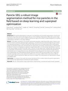
detection. (d) Using Gauss-Laplace filter to detection. (e) Using traditional morphology filter to detection. (f) Our proposed method to detection.

(1)

−∞

where, p(x) is the probability of occurrence x. In an original image, set T as the threshold. If the pixel greys level less than T, it is an object. Otherwise, it is the background. pi is

3. Adaptive Fuzzy C-Means

the probability of grey level at pixel i, the probability of objects and background respectively as,

If the gray level of the target and background is highly correlated, the gradient value in each target region and background region is smaller than that at edge region. That is to say, the pixel value of target and background is close to the gradation axis in the gradation-gradient-two dimensional coordinate plane. While the edge region stay away from the gray axis. Furthermore, the edge regions are definitely between the background and targets or between different targets. We can abandon the larger gradient value pixels, which can filter the image. See Fig.2, the gradation-gradient coordinate plane.

T −1

po = ∑ pi , i = 1,2,, T − 1;

(2)

i =0

255

pb = ∑ pi , i = T , T + 1,,255;

(3)

i =T

Then, we get the entropy of object and background as

H o (T ) = −∑ ( pi / po ) lg( pi / po ) i = 0,1,2,, T − 1;

(4)

H b (T ) = −∑ ( pi / pb ) lg( pi / pb ) i = T , T + 1,,255;

(5)

i

i

The entropy of image is

H (T ) = H o (T ) + H b (T )

gradient

(6)

edge edge background object

gradation

Fig. 2. Gradation-gradient two-dimensional histogram. In the clustering algorithm, the number of clusters is often given as the initial conditions, which can realize the unknown data categories and give a clustering algorithm for estimating the numbers of objects. If inappropriate choice of cluster number, it will make the mismatch between the results of the division data sets and real data sets, leading to a failure of cluster. In this paper, we propose the gradation-gradient-two dimensional histogram coordinate plane for deciding the objects in an image. In this histogram, according to the number of peaks to determine the number of clusters to complete clustering unsupervised. Let f(x,y) as an image, x, y represent the location of the image. The gradient value of each pixel is defined as

[

∇f = G x2 + G y2

]

1/ 2

=

[(

) +( ) ]

∂f 2 ∂x

1/ 2 ∂f 2 ∂y

(7)

Set the pixel number as NAB, which with a gray level A and gradient value B. Then the gradation-gradient histogram is

H AB = N AB / N

(8)

where N is the all pixel number of the image. We set the gradation-gradient threshold to remove the high gradient

Fig. 1. (a) Original image with noise. (b) Granularity detection with Gauss noise. (c) Using Sobel filter to

41

pixels in the gradation-gradient histogram. And then, make a projection to gradation, forming one-dimensional histogram h(x). After that, make a convolution of h(x) and g(x). ∞

Φ ( x) = h( x) ∗ g ( x) = ∫ h(u ) −∞

Where,

g ( x) =

1 2π σ

exp[−

1 2π σ

exp[−

The ACWFCM objective function (10) is minimized when high membership values are assigned to pixels whose intensities are close to the centroid for its particular class, and low membership values are assigned where the pixel data is far from the centroid. The advantage of ACWFCM is that if a pixel is corrupted by strong noise, then the segmentation will be only changed with some fractional amount .But in hard segmentations, the entire classification may change. Meanwhile, in the segmentation of images, fuzzy membership functions can be used as an indicator of partial volume averaging, which occurs where multiple classes are present in a single pixel. Furthermore, the improved algorithm can remove noise, get the number of clusters more accurately, and obtain a better segment result. The objective function JACWFCM can be minimized in a fashion similar to the standard FCM algorithm. The steps for our ACWFCM algorithm can be described as follows: Step 1. Provide initial values for centroids, vk, k=1... C and C is automatically defined by function (2.4). Step 2. Compute new memberships as follows:

( x − u) 2 ]du (9) 2σ 2

( x − u ) 2 . The number of ] 2σ 2

cluster C can be automatically calculated by the aggregate

{xi | Φ ' ( xi ) = 0, Φ " ( xi ) < 0} . The centroids v k are {xi } .

C  {x i | Φ ' ( x i ) = 0, Φ " ( x i ) < 0}

(10)

3.1 ACWFCM Algorithm In this section, we propose a new objective function for obtaining fuzzy segmentations of images with automatically determine the cluster number C. The ACWFCM algorithm for scalar data seeks the membership functions u k and the centroids v k , such that the following objective function is minimized:

J ACWFCM = where

C

∑ ∑w u

( x , y ),i∈N k =1

i

k

u k ( x, y ) =

( x, y ) || I ( x, y ) − v k || (11) q

2

∑

C k =1

u k ( x, y ) = 1 , I(x,y) is the

observed image intensity at location (x,y), and vk is the centroid of class k. The total number of class C is automatically calculated by function (10). The parameter q is a weighting exponent on each fuzzy membership and determines the amount of fuzziness of the resulting classification. For simplicity, we assume for the rest of this paper that q=2 and the norm operator || ⋅ || represents the standard Euclidean distance. The main role of weighting parameter wi is adjusting the cluster centers. wi can be

vk

__

__

and f (x,y). In the two dimensional gradation histogram, H(s,t) expresses the joint probability density, which with the gray level s at source image f(x,y) and with gray level t __

at smooth image f (x,y).

where,

∑

N

i =1

(13)

∑ =

x, y

wi u k ( x, y ) 2 I ( x, y )

∑

w u ( x, y ) 2 x, y i k

(14)

k=1... C and 0 < i ≤ N . Step 4. If the algorithm has converged, then quit. Otherwise, go to Step 2. In practice, we used a threshold value of 0.001. 3.2 Experiments and Discussions We implemented ACWFCM on a Core2 2.0GHz processor using MATLAB. Execution time for ACWFCM ranged from 2 seconds to 5 seconds for a 256☓256 image. For comparison, the first experiment applies the Otsu and FCM methods to segment the brain image. In the second experiment, we take the ACWFCM for segmenting. Fig.3 (b) to (d) shows the results of applying the Otsu method, FCM and ACWFCM algorithms to segment. The noise of Otsu and FCM are appeared clearly, but there is less noise in ACWFCM. People set different cluster number C, people can get different results. Fig.4 is FCM segmentation methods with different C. But, the ACWFCM method can automatic get the cluster number C without people set. So,

calculated by source image f(x,y) and smooth image f (x,y). n expresses the times of pixel (x,y) appeared in the image. We form a two dimensional gradation histogram by f(x,y)

wi = H ( s, t )

∑l =1|| I ( x, y) − vl || −2 /( q−1) C

For all (x,y), k=1,...,C and q=2. Step 3. Computer new centroids as follows:

u k ( x, y ) is the membership value at pixel location

(x,y) for class k such that

|| I ( x, y ) − v k || −2 /( q −1)

(12)

wi = 1 , N is the all pixel number of the image

[22]. When wi=1/N, that is to say, the same effect to the classification of each class, ACWFCM is degenerated to the standard FCM.

42

the ACWFCM segment result is better than other methods.

(a)Brain image.

(g) c=8 (h) c=9 Fig. 4. FCM segmentation methods with different C

(b) Otsu segment image.

4. Level Set Method Level Set Method. In Chan-Vese Model, set an image u0(x,y). Given the curve C = ∂w , with w ⊂ Ω an open subset, and two unknown constants c1 and c2. Denoting

Ω1 = w , Ω 2 = Ω \ w , the energy function is

F (c1 , c2 , C ) = µ ⋅ Length(C ) + ν ⋅ Area(inside(C )) (15) (c) FCM segment image. (d) ACWFCM segment image. Fig. 3. Results of different segment methods.

+ λ1 ∫

Ω1 = w

| u0 − c1 |2 dxdy

+ λ2 ∫

Ω 2 =Ω \ w

| u0 − c2 |2 dxdy

μ ≥ 0, ν ≥ 0, λ1 , λ2 > 0 are fixed parameters. In almost calculations, we fix λ1 = λ2 = 1 and ν = 0 . If and

where

only if the curve C on the boundary of homogeneity area, the above function obtain minimum value. Set φ as the level

(a) c=2

set function. Then, the energy F (c1 , c 2 , φ ) can be written as F (c1 , c 2 , φ ) = µ ∫ δ (φ ) | ∇φ | dxdy + ν ∫ H (φ )dxdy + Ω Ω (16) λ1 ∫ | u 0 − c1 | 2 H (φ )dxdy

(b) c=3

Ω

+ λ 2 ∫ | u 0 − c 2 | 2 (1 − H (φ ))dxdy Ω

φ

Keeping

fixed

and

minimizing

the

energy

F (c1 , c2 , φ ) with respect to the constants c1 and c2, we can get the following formulas with C = {( x, y ) | φ ( x, y ) = 0} (c) c=4

c1 =

(d) c=5

∫u Ω

0

( x, y ) H (φ ( x, y ))dxdy

∫

Ω

c2 =

∫u Ω

0

H (φ ( x, y ))dxdy

( x, y )(1 − H (φ ( x, y )))dxdy

∫ (1 − H (φ ( x, y)))dxdy Ω

∂φ = δ (φ ) µ∇ ∂t

[ ( ) −ν − λ (u

Where, (e) c=6

(f) c=7

δ( z) = 43

∇φ |∇φ |

1

Heaviside

dH ( z ) dz

is

0

functions

Dirac

]

− c1 ) 2 + λ2 (u 0 − c2 ) 2 (17)

H ( z ) = 1 z ≥ 0 . 0 z < 0

function.

In

practice,

H ε ( z ) = 12 (1 + π2 arctan( εz )) and δε ( z ) = π1 ⋅ ε 2 +ε z 2 where ε is constant.

To

,

∂φ ∂t

= δ ε (φ )div(

∇φ |∇φ |

form

of

function

(18),

) can be written by the semi-implicit

AOS scheme as

Fast Implicit Level Set Method. From the function, we can found that the main force level set evolution is

φin+1 = φin + τδ (φi )

depended on − λ1 (u 0 − c1 ) + λ2 (u 0 − c 2 ) . As we set 2

simplified

2

2 (φ jn +1 − φin +1 ) (20) n j∈N ( i ) (| ∇φ |) + (| ∇φ |) j

∑

n i

λ1 = λ2 = 1 , decompose it by squared difference formula,

Note that by evaluating only image positions with

− c2 )(u 0 − c1 +2c2 ) . Then, we propose the

| ∇φ |i ≠ 0 , the denominator in this scheme cannot vanish.

we can get 2(c1

following model [31] c +c  ∂φ  (18) =| ∇φ |  u 0 − 1 2  ∂t 2   This function is ordinary differential equation (ODE). Where, δ ε ( x) =| ∇φ | , which in order to increasing the scope of force level set evolution.

u0 −

c1 + c2 2

In matrix-vector notation this becomes

  φ n+1 = φ n + τ  ∑ Al (φ n ) φ n+1  l∈{x , y} 

(21)

where Al describes the interaction in l direction. x, y respectively the x-direction and y-direction (2D). With the definition of Al (ϕn) = aij(ϕn), and aij(ϕn) can be expressed as

is the speed

term.

δ (φi ) (|∇φ |) n +2 (|∇φ |) n , j ∈ N l (i ) i j  aij = 0, else − δ (φ ) 2 i (|∇φ |) n + (|∇φ |) n , i = j  i j

(22)

According to above equations, the formulation (4.6) can be re-expressed as

φ n+1 =

)

(23)

So, combine with formulation (22), the formulation (23) finally can be written as

Fig.5. Evolution of the curve C in the image. In Fig.5, ''+'' and ''-'' represent the sign of speed term, ''→'' is the motivation of the curve C. We can see that according Hamilton-Jacobi partial differential equation, the curve C will eventually stop in the target's boundary. A given curve C is represented implicitly, as the zero level set of a scalar Lipschitz continuous function ϕ, such that (see Fig.5):

 φ < 0 in w  φ > 0 in Ω \ w φ = 0 on ∂w 

(

−1 1 I − 2τAl (φ n ) φ n ∑ 2 l∈{ x , y}

φ1n +1 =| ∇φ1n | {

(

(

1 2 ∑ I − 2τµAl (φ1n ) 2 l =1

)H (φ

(

× [φ1n − u 0 −

c11 + c01 2

φ 2n +1 =| ∇φ 2n | {

1 2 ∑ I − 2τµAl (φ 2n ) 2 l =1

(

n 2

) + u0 −

(

)

(

)

−1

c10 + c00 2

)(1 − H (φ ))]} n 2

)

−1

(24)

)(

)

× [φ 2n − u 0 − c11 +2c10 H (φ1n ) + u 0 − c01 +2c00 1 − H (φ1n ) ]}

The imaging system is ultimately based on hardware. The choice of detectors, amplifiers, and sampling methods plays an important role in overall performance. Image degradation can be caused by deficiencies in the imaging hardware. In this paper, we compare our method with [33]. The proposed improved implicit active contour model has been applied to a variety of synthetic and real images. The results calculated on a standard personal computer with Windows XP, Intel Core 2.0 GHz, 1G RAM, λ1 = λ2 = 1 ,

(19)

In this study, we use a semi-implicit additive operator splitting (AOS) method rather than explicit schemes to implement the discrete level set processing. The basic idea of the AOS scheme is to split the m-dimensional spatial operator into a set of one-dimensional space discretization’s that can be efficiently solved with Gaussian elimination algorithm named Thomas Algorithm.

µ = 0.1× 255 2 , ν = 0

. During the experiments, we compare the results with iterations, CPU time and segmentation results. The results are shown in Fig. 6. In this experiment, the segmentation results are the same. However, our algorithm iterate 7 times, cost CPU 44

time 0.72 sec. Use traditional level set method, it iterated 500 times, cost CPU time 39.25 sec. We can briefly see that our method is better.

granularity analysis method and morphology method to recognize the blood cancer cells in bone marrow. The system is proved more efficient than traditional systems. We developed a new theoretical approach to automatically selecting the weighting exponent in the FCM to segment the brain images. The experimental results illustrate the effectiveness of the proposed method. We propose a new image segment method for X-ray lesions inspection systems. The Fast Level Set Method (FLSM) scheme eliminates the need of re-initialization and speed up the computational complexity. Beside of this, the new inspection technology has the advantages of high performance, excellent radiation safety and good reliability, cheaper price and smaller floor area, easy operation and maintenance and so on. The enhancement gives specific regions of concern through real-time screen updates driven by sliding a finger on the touchpad. The new imaging modalities, used in combination with thoughtfully develop detector electronics.

(a) DR image of brain image after pre-processing

References [1].Nigel Gilbert, Researching Social Life 3rd Edition, SAGE Press, London, 2010. [2].G. Longford, The social impact of information technology on daily life, Canadian Journal of Cultural Studies, 2006. [3].J.S. Brown, and P. Duguid, The Social Life of Information, Harvard Business School Press, 2002. [4].R.C. Gonzalez, and R.E. Woods, Digital Image Processing, 2nd Edition, Prentice Hall, 2008. [5].M. Kass, A. Witkin, D. Terzopoulos, Snakes: Active contour models, International Journal of Computer Vision, vol.1, no.4 (1998), p.321. [6].V.G. Leticia, A.A. Suzim, J. Maeda, A new automatic circular decomposition algorithm applied to blood cells image, IEEE Computer Society, (2000), p.277-280. [7].N. Sinha, A.G. Ramakrishnan, Automation of differential blood count, Digital Object Identifier, vol.2, no.15-17(2003), p.547-551. [8].Y. Cong, L. Qiuping, F. Nianlun, Microscopic image analysis and recognition on pathological cells, Journal of Biomedical Engineering Research, vol.28, no.1(2009), p.35-38. [9].H. Zhoujie, M. Shoushi, P. Xichun, P. Xin, Studies on the recognition of marrow cell image, Computing Technology and Automation, vol.24, no.3 (2005). [10].J. Debayle, and J.C. Pinoli, Multi-scale image filtering

(b) FLSM segmentation of fig.6(a) Fig.6. The DR brain image segmentation with FLSM scheme.

5. Conclusions Medical image segmentation is the key steps of medical image processing and analysis. It occupies important position in medical image project. Many classical image segmentation algorithms have appeared, but there are still not a general algorithm can successfully complete image segmentation. In order to solve these segmentation problems, people constantly introducing new methods and new theory which make medical image segmentation become a popular research fields. We firstly adopted 45

and segmentation by menas of adaptive neighborhood mathematical morphology, Proceeding of IEEE International Conference on Image Processing, Genova, Italy, vol.3(2005), p.537-540. [11].T. Xuemin, L. Xueyin, H. Lin, Research on automatic recognition system for leucocyte image, Journal of Biomedical Engineering, vol.24, no.6 (2007), p.1250-1255. [12].B. Funt, K. Bernard, L. Martin, Is machine color constancy good enough, Proceeding of the 5th European Conference on Computer Vision, Freiburg, Germany, (1998), p.445-459. [13].H. Lu, L. Zhang, S. Serikawa, A method for infrared image segmentation based on sharp frequency localized contourlet transform and morphology, Proceeding of International Conference on Intelligent Control and Information Processing, Dalian, China, (2010), p.79-82. [14].Y. Li, L. Zhang, H. Lu, S. Serikawa, An improved detection algorithm based on morphology methods for blood cancer cells detection, Journal of Computational Information Systems, vol.7, no.13 (2011), p.4724-4731. [15].Y. Li, L. Zhang, H. Lu, S. Serikawa, A new type of using morphology methods to detect blood cancer cells, Proceeding of LNCS CCIS, Part I, vol.182(2011), p.16-23. [16].C.W. Chen, J. Luo, and K.J. Parker, Artifact reduction in low bit rate DCT-based image compression, IEEE Trans. on Image Processing, vol.7, no.12 (1998), p.1673-1683. [17].J. Han, M. Kamber, Data mining: Concepts and Techniques, Morgan Kaufmann Publishers, 2001. [18].B. Otman, Z. Hongwei, K. Fakhri, Connectionist-based dempster shafer evidential reasoning for data fusion, Fuzzy Based Image Segmentation, Springer-Verlag, Berlin, 2003. [19].S. Shen, W.A. Sandham, Fuzzy clustering based applications to medical image segmentation, Proceeding of the 25th Annual International Conference on the IEEE EMBS, Cancun, UK, (2003), p.747-750. [20].M. Hung, D. Yang, An efficient fuzzy c-means clustering algorithm, Proceeding of International Conference on Data Mining, (2001), p.225-232. [21].J.X. Sun, Image Processing, Science Press, 2005. [22].G. Xinbo, L. Jie, J. Hongbing, A multi-threshold image segmentation algorithm based on weighting fuzzy c-means clustering and statistical test. Acta Electronic Sinica, vol.32, no.4 (2004), p.661-664. [23].Y. Li, H. Lu, B. Li, and S. Serikawa, An automatic image segmentation algorithm based on weighting fuzzy c-means clustering, Proceeding of LNCS CCIS, Part I, vol.182(2011), pp.24-29. [24].L. Chen, H.D. Cheng, J. Zhang, Fuzzy subfiber and its

application to seismic lithology classification, information science, vol.1, no.2(1994), p.77-95. [25].J. Shi, and J. Malik, Normalized cuts and image segmentation, IEEE Trans. on Pattern Analysis and Machine Intelligence, vol.22, no.8 (2000), p.888-905. [26].M. Pathegama, Edge-end pixel extraction for edge-based image segmentation, Trans. on Engineering Computing and Technology, vol.2,(2004), p.213-216. [27].L.G. Shapiro, and G.C. Stockman, Computer Vision, Prentice Hall, 2001. [28].S. Osher, and N. Paragios, Geometric level set methods in imaging vision and graphics, Springer Verlag, 2003. [29].K. Kang, Recent developments and applications of radiation/detection technology in Tsinghua university, Nuclear Physics, vol.A-834, (2010), p.736c-742c. [30].T.F. Chan, L. A. Vese, Active contours without edges, IEEE Trans. on Image processing, vol.10, no.2(2001), p.266-277. [31].H. Lu, S. Serikawa, Y. Li, Proposal of fast implicit level set scheme for medical image segmentation using the chan and vese model, Applied Mechanics and Materials, vol.103 (2012), p.695-699. [32].G. Kuhne, J. Weickert, Fast implicit active contour models, Lecture Notes in Computer Science, (2002), p.133-140. [33].S. Qi, C. Peng, C. Jingyun, Image segmentation based on level set method in luggage inspection system, Atomic Energy Science and Technology, vol.40, no.6(2006), p.745-748. [34].Y. Li, H. Lu, S. Serikawa, Image Segmentation based on improved fast implicit level set scheme in x/γ-ray inspection system, Applied Mechanics and Materials, vol.103(2012), p.705-710.

46